
Appendix B
Attenuation, Phase Shift and Decibels
The transfer function of a linear time-invariant system, denoted by H(ω), is in general a complex function of ω. It is indicative of the manner in which time harmonic signals (sine and cosine) propagate through such a system. The modulus of H(ω) is the factor by which the amplitude of the incoming harmonic signal is scaled and the argument of H(ω) indicates the phase shift introduced by the system. We then can write
![]()
where
![]()
is the attenuation of the system in neper (abbreviated as Np) and b(ω) is the phase shift introduced by the system. The neper is an old unit that is not used in practice anymore. A more common measure of attenuation is the decibel (abbreviated as dB). The attenuation in dB is defined as
![]()
From the relation
![]()
we conclude that
![]()
From this it follows that 1 Np is equivalent to 8.686 dB. Because the neper is used infrequently, we will drop the subscript ‘d’ and henceforth speak about attenuation exclusively in terms of dB and denote this as a. The transfer function H(ω) is usually defined as a ratio of the output voltage (or current) and the input voltage (or current). If we look at the power ratio between the input and output, it is evident that the powers are proportional to the square of the voltages or currents, i.e.
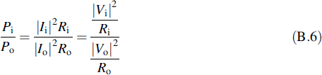
where the indices ‘o’ and ‘i’ indicate that the quantity is related to the output and input, respectively. The quantities Ro,i give the real part of the impedances. If we assume the situation where Ro = Ri, which is often the case, then the power attenuation is found as
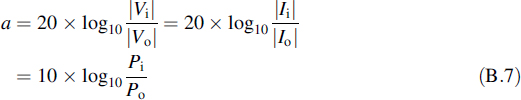
The advantage in using a logarithmic measure for the ratio of magnitudes between the inputs and outputs lies in the fact that in series connections of systems, the attenuation in each of the systems expressed in dB needs only to be summed in order to obtain the total attenuation in dB.
Furthermore, we mention that the decibel is also used to express the absolute levels of power, current and voltage. The following notations are among others in use:
- dBW - power with respect to P0 = 1 W
- dBm - power with respect to P0 = 1 mW
- dBμV - voltage with respect to V0 = 1 μV.
Definitions and general properties of logarithms are given in Appendix C, Section C.6. Table B.1 presents a list of linear power ratios and the corresponding amount of dBs.
Table B.1 List of dB values for a given linear power ratio
| Linear ratio | dB |
| 0.25 | −6 |
| 0.5 | −3 |
| 1 | 0 |
| 2 | 3 |
| 4 | 6 |
| 10 | 10 |
| 100 | 20 |
| 1000 | 30 |
Introduction to Random Signals and Noise W. van Etten © 2005 John Wiley & Sons, Ltd