Appendix A

Representation of Signals in a Signal Space

A.1 LINEAR VECTOR SPACES

In order to facilitate the geometrical representation of signals, we treat them as vectors. Indeed, signals can be considered to behave like vectors, as will be shown in the sequel. For that purpose we recall the properties of linear vector spaces. A vector space is called a linear vector space if it satisfies the following conditions:

where x and y are arbitrary vectors and α and β are scalars.

In an n-dimensional linear vector space we define a so-called inner product as

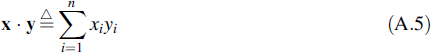
where x_i and y_i are the elements of x and y, respectively. Two vectors x and y are said to be orthogonal if x · y = 0. The norm of a vector x is denoted by || x || and we define it by

This norm has the following properties:

In general, we can state that the norm of a vector represents the distance from an arbitrary point described by the vector to the origin, or alternatively it is interpreted as the length of the vector. From Equation (A.9) we can readily derive the Schwarz inequality

A.2 THE SIGNAL SPACE CONCEPT

In this section we consider signals defined on the time interval [a, b]. As in the case of vectors, we define the inner product of two signals x(t) and y(t), but now the definition reads

Note that using this definition, signals behave like vectors, i.e. they show the properties 1 to 8 as given in the preceding section. This is readily verified by considering the properties of integrals.

Let us consider a set of orthonormal signals {ϕ_i(t)}, i.e. signals that satisfy the condition

where δ_ij denotes the well-known Kronecker delta. When all signals of a specific class can exactly be described as a linear combination of the members of such a signal set, we call it a complete orthonormal signal set; here we take the class of square integrable signals. In this case each arbitrary signal of that class is written as

and the sequence {s_i} can also be written as a vector s, where the s_i are the elements of the signal vector s. Figure A.1 shows a circuit that reconstructs s(t) from the set {s_i} and the orthonormal signal set {ϕ_i(t)}; this circuit follows immediately from Equation (A.14).

No limitations are placed on the integer n; even an infinite number of elements is allowed. The elements s_i are found by

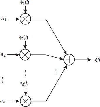
Figure A.1 A circuit that produces the signal s(t) from its elements {s_i} in the signal space

Figure A.2 A circuit that produces the signal space elements {s_i} from the signal s(t)

Therefore, when we construct a vector space using the vector s, we have a geometrical representation of the signal s(t). Along the ith axis we imagine the function ϕi(t); i.e. the set {ϕ_i(t)} is taken as the basis for the signal space. In fact, s_i, indicates to what extent ϕ_i(t) contributes to s(t). From Equation (A.15) a circuit is derived that produces the elements {s_i} representing the signal s(t) in the signal space {ϕ_i(t)}; the circuit is given in Figure A.2.

The inner product of a signal vector with itself has an interesting interpretation:

with E_s the energy of the signal s(t). From this equation it is concluded that the length of a vector in the signal space equals the square root of the signal energy. For purposes of detection it is important to establish that the distance between two signal vectors represents the square root of the energy of the difference of the two signals involved.

This concept of signal spaces is in fact a generalization of the well-known Fourier series expansion of signals.

A.3 GRAM-SCHMIDT ORTHOGONALIZATION

When we have an arbitrary set {f_i(t)} of, let us say, N signals, then in general these signals will not be orthonormal. The Gram-Schmidt method shows us how to transform such a set into an orthonormal set, provided the members of the set {f_i(t)} are linearly independent, i.e. none of the signal f_i(t) can be written as a linear combination of the other signals. The first member of the orthonormal set is simply constructed as

In fact, the signal f₁(t) is normalized to the square root of its energy, or equivalently to the length of its corresponding vector in the signal space.

The second member of the orthonormal set is constructed by taking f₂(t) and subtracting from this f₂(t) the part that is already comprised of ϕ₁(t). In this way we arrive at the intermediate signal

Due to this operation the signal g₂(t) will be orthogonal to ϕ₁(t). The functions ϕ₁(t) and ϕ₂(t) will become orthonormal if we construct ϕ₂(t) from g₂(t) by normalizing it by its own length:

Proceeding in this way we construct the kth intermediate signal by

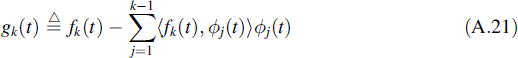
and by proper normalization we arrive at the kth member of the orthonormal signal set

This procedure is continued until N orthonormal signals have been constructed. In case there are linear dependences, the dimensionality of the orthonormal signal space will be lower than N.

The orthonormal space that results from the Gram-Schmidt procedure is not unique; it will depend on the order in which the above described procedure is executed. Nevertheless, the geometrical signal constellation will not alter and the lengths of the vectors are invariant to the order chosen.

A.4 THE REPRESENTATION OF NOISE IN SIGNAL SPACE

In this section we will confine our analysis to the widely used concept of wide-sense stationary, zero mean, white, Gaussian noise. A sample function of the noise is denoted by N(t) and the spectral density is N₀/2. We construct the noise vector n in the signal space, where the elements of this noise vector are defined by

Since this integration is a linear operation, these noise elements will also show a Gaussian distribution and it will be clear that the mean of n_i, equals zero, for all i. When, besides these data, the cross-correlations of the different noise elements are determined, the noise elements are completely specified. Those cross-correlations are found to be

Figure A.3 The construction of a set of orthonormal functions {ϕ_i,(t)} from a set of given functions {f_i(t)} using the Gram-Schmidt orthogonalization procedure

elements are completely specified. Those cross-correlations are found to be

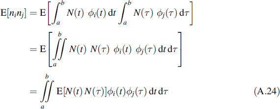
In this expression the expectation represents the autocorrelation function of the noise, which reads R_NN(t, τ) = δ(t − τ)N₀/2. This is inserted in the last equation to arrive at

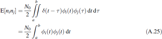
Remembering that the set {ϕ_i(t)} is orthonormal, the following cross-correlations result

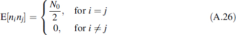
From this equation it is concluded that the different noise elements n_i are uncorrelated and, since they are Gaussian with zero mean, they are independent. Moreover, all noise elements show the same variance of N₀/2. This simple and symmetric result is another interesting feature of the orthonormal signal spaces as introduced in this appendix.

A.4.1 Relevant and Irrelevant Noise

When considering a signal that is disturbed by noise we want to construct a common signal space to describe both the signal and noise in the same space. In that case we construct a signal space to completely describe all possible signals involved. When we want to attempt to describe the noise N(t) using that signal space, it will, as a rule, be inadequate to completely characterize the noise. In that case we split the noise into one part N_r(t) that is projected on to the signal space, called the relevant noise, and another part N_i(t) that is orthogonal to the space set up by the signals, called the irrelevant noise. Thus, the relevant noise is given by the vector n_r with components

By definition the irrelevant noise reads

Next we will show that the irrelevant noise part is orthogonal to the signal space. For this purpose let us consider a signal s(t) and an orthonormal signal space {ϕ_i(t)}. Let us suppose that s(t) can completely be described as a vector in this signal space. The inner product of the irrelevant noise N_i(t) and the signal reads

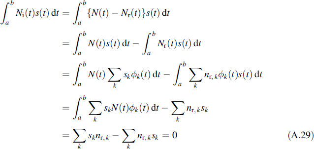
For certain applications, for instance optimum detection of a known signal in noise, it appears that the irrelevant part of the noise may be discarded.

A.5 SIGNAL CONSTELLATIONS

In this section we will present the signal space description of a few signals that are often met in practice. The signal space with indications of possible signal realizations is called a signal constellation. In detection, the error probability appears always to be a function of E_d/N₀, where E_d is the energy of the difference of signals. However, we learned in Section A.2 that this energy is in the signal space represented by the squared distance of the signals involved. Considering two signals s_i(t) and s_j(t), their squared distance is written as

where E_i and E_j are the energies of the corresponding signals and E_ij represents the inner product of the signals. In specific cases where E_i = E_j, = E for all i and j, Equation (A.30) is written as

with the cross-correlations ρ_ij defined by

A.5.1 Binary Antipodal Signals

Consider the two rectangular signals

and their bandpass equivalents

with T = n × 2π/ω₀ and n integer.

The cross-correlation of those signals equals − 1 and the distance between the two signals is

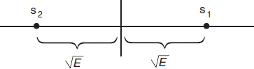
Figure A.4 The signal constellation of the binary antipodal signals

The space is one-dimensional, since the two signals involved are dependent. The signal vectors are and . This signal set is called an antipodal signal constellation and is depicted in Figure A.4.

A.5.2 Binary Orthogonal Signals

Next we consider the signal set

where either T = nπ/ω (with n integer) or T 1/ω₀, so that ρ₁₂ = 0 or ρ₁₂ ≈ 0, respectively. Due to this property those signals are called orthogonal signals. In this case the signal space is two-dimensional and , while . It is easily verified that the distance between the signals amounts to . The signal constellation is given in Figure A.5.

Figure A.5 The signal constellation of the binary orthogonal signals

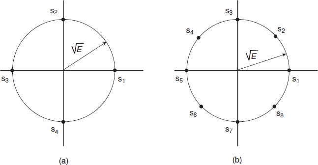
Figure A.6 The signal constellation of M-phase signals

A.5.3 Multiphase Signals

In the multiphase case all possible signal vectors are on a circle with radius . This corresponds to the M-ary phase modulation. The signals are represented by

with the same requirement for the relation between T and ω₀ in the former section. The signal vectors are given by

In Figure A.6 two examples are depicted, namely M = 4 in Figure A.6(a) and M = 8 in Figure A.6(b). The case of M = 4 can be considered as a pair of two orthogonal signals; namely the pair of vectors [s₁,s₃] is orthogonal to the pair [s₂,s₄]. For that reason this is a special case of the biorthogonal signal set, which is dealt with later on in this section. This orthogonality is used in QPSK modulation.

A.5.4 Multiamplitude Signals

The multiamplitude case is a straightforward extension of the antipodal signal constellation. The extension is in fact a manifold, let us say M, of signal vectors on the one-dimensional axis (see Figure A.4). In most applications these points are equidistant.

Figure A.7 The signal constellation of QAM signals: (a) rectangular distribution; (b) circular distribution

A.5.5 QAM Signals

A QAM (quadrature amplitude modulated) signal is a signal where both the amplitude and phase are modulated. In that sense it is a combination of the multiamplitude and multiphase modulated signal. Different constellations are possible; two of them are depicted in Figure A.7. Figure A.7(a) shows a rectangular grid of possible signal vectors, whereas in the example of Figure A.7(b) the vectors are situated on circles. This signal constellation is used in such applications as high-speed telephone modems, cable modems and digital distribution of audio and video signals over CATV networks.

A.5.6 M-ary Orthogonal Signals

The M-ary orthogonal signal set is no more no less than an M-dimensional extension of the binary orthogonal signal set; i.e. in this case the signal space has M dimensions and all possible signals are orthogonal to all others. For M = 3 and assuming that all signals bear the same energy, the signal vectors are

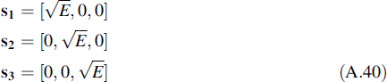
This signal set has been illustrated in Figure A.8. The distance between two arbitrary signal pairs is .

A.5.7 Biorthogonal Signals

An M-ary biorthogonal signal set is constructed from an M/2-ary orthogonal signal set by simply adding the negatives of all the orthogonal signals. It will be clear that the dimension of the signal space remains as M/2. The result is given in Figure A.9(a) for M = 4 and in Figure A.9(b) for M = 6.

Figure A.8 The signal constellation of the M-ary orthogonal signal set for M = 3

Figure A.9 The signal constellation of the M-ary biorthogonal signal set for (a) M = 4 and (b) M = 6

A.5.8 Simplex Signals

To explain the simplex signal set we start from a set of M orthogonal signals {f_i(t)} with the vector presentation {f_i}. We determine the mean of this signal set

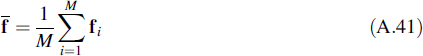
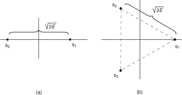
Figure A.10 The simplex signal set for (a) M = 2 and (b) M = 3

In order to arrive at the simplex signal set, this mean is subtracted from each vector of the orthogonal set:

In fact this operation means that the origin is translated to the point f. Therefore the distance between any pair of possible vectors s_i, remains . Figure A.10 shows the simplex signals for M = 2 and M = 3. Note that the dimensionality is reduced by 1 compared to the starting orthogonal set.

Due to the transformation the signals are no longer orthogonal. On the other hand, it will be clear that the mean signal energy has decreased. Since the distance between signal pairs are the same as for orthogonal signals, the simplex signal set is able to realize communication with the same quality (i.e. error probability) but using less energy per bit and thus less power.

A.6 PROBLEMS

A.1 Derive the Schwarz inequality (A.11) from the triangular inequality (A.9).

A.2 Use the properties of integration and the definition of Equation (A.12) to show that signals satisfy the properties of vectors as given in Section A.1.

A.3 Use Equation (A.19) to show that g₂(t) is orthogonal to ϕ₁(t).

A.4 Show that for binary orthogonal signals one of the two given relations between T and ω₀ is required for orthogonality.

A.5 Calculate the distance between adjacent signal vectors, i.e. the minimum distance, for the M-ary phase signal.

A.6 Calculate the energy of the signals from the simplex signal set, expressed in terms of the energy in the signals of the M-ary orthogonal signal set.

A.7 Calculate the cross-correlation between the various signals of the simplex signal set.