
1
Introduction
1.1 RANDOM SIGNALS AND NOISE
In (electrical) engineering one often encounters signals that do not have a precise mathematical description, since they develop as random functions of time. Sometimes this random development is caused by a single random variable, but often it is a consequence of many random variables. In other cases the causes of randomness are not clear and a description is not possible, but the signal is characterized by means of measurements only.
A random time function may be a desired signal, such as an audio or video signal, or it may be an unwanted signal that is unintentionally added to a desired (information) signal and disturbs the desired signal. We call the desired signal a random signal and the unwanted signal noise. However, the latter often does not behave like noise in the classical sense, but it is more like interference. Then it is an information bearing signal as well, but undesired. A desired signal and noise (or interference) can, in general, not be distinguished completely; by means of well-defined signal processing in a receiver, the desired signal may be favoured in a maximal way whereas the disturbance is suppressed as much as possible. In all cases a description of the signals is required in order to be able to analyse its impact on the performance of the system under consideration. Especially in communication theory this situation often occurs. The random character as a function of time makes the signals difficult to describe and the same holds for signal processing or filtering. Nevertheless, there is a need to characterize these signals by a few deterministic parameters that enable the system user to assess the performance of the system. The tool to deal with both random signals and noise is the concept of the stochastic process, which is introduced in Section 1.3.
This book gives an elementary introduction to the methods used to describe random signals and noise. For that purpose use is made of the laws of probability, which are extensively described in textbooks [1–5].
1.2 MODELLING
When studying and analysing random signals one is mainly committed to theory, which however, can be of good predictive value. Actually, the main activity in the field of random signals is modelling of processes and systems. Many scientists and engineers have contributed to that activity in the past and their results have been checked in practice. When a certain result agrees (at least to a larger extent) with practical measurements, then there is confidence in and acceptance of the result for practical application. This process of modelling has schematically been depicted in Figure 1.1.

Figure 1.1 The process of modelling
In the upper left box of this scheme there is the important physical process. Based on our knowledge of the physics of this process we make a physical model of it. This physical model is converted into a mathematical model. Both modelling activities are typical engineer tasks. In this mathematical model the physics is no longer formally recognized, but the laws of physics will be included with their mathematical description. Once the mathematical model has been completed and the questions are clear we can forget about the physics for the time being and concentrate on doing the mathematical calculations, which may help us to find the answers to our questions. In this phase the mathematicians can help the engineer a lot. Let us suppose that the mathematical calculations give a certain outcome, or maybe several outcomes. These outcomes would then need to be interpreted in order to discover what they mean from a physical point of view. This ends the role of the mathematician, since this phase is maybe the most difficult engineering part of the process. It may happen that certain mathematical solutions have to be discarded since they contradict physical laws. Once the interpretation has been completed there is a return to the physical process, as the practical applicability of the results needs to be checked. In order to check these the quantities or functions that have been calculated are measured. The measurement is compared to the calculated result and in this way the physical model is validated. This validation may result in an adjustment of the physical model and another cycle in the loop is made. In this way the model is refined iteratively until we are satisfied about the validation. If there is a shortage of insight into the physical system, so that the physical model is not quite clear, measurements of the physical system may improve the physical model.
In the courses that are taught to students, models that have mainly been validated in this way are presented. However, it is important that students are aware of this process and the fact that the models that are presented may be a result of a difficult struggle for many years by several physicists, engineers and mathematicians. Sometimes students are given the opportunity to be involved in this process during research assignments.
1.3 THE CONCEPT OF A STOCHASTIC PROCESS
In probability theory a random variable is a rule that assigns a number to every outcome of an experiment, such as, for example, rolling a die. This random variable X is associated with a sample space S, such that according to a well-defined procedure to each event s in the sample space a number is assigned to X and is denoted by X(s). For stochastic processes, on the other hand, a time function x(t, s) is assigned to every outcome in the sample space. Within the framework of the experiment the family (or ensemble) of all possible functions that can be realized is called the stochastic process and is denoted by X(t, s). A specific waveform out of this family is denoted by xn(t) and is called a sample function or a realization of the stochastic process. When a realization in general is indicated the subscript n is omitted. Figure 1.2 shows a few sample functions that are supposed to constitute an ensemble. The figure gives an example of a finite number of possible realizations, but the ensemble may consist of an infinite number of realizations. The realizations may even be uncountable. A realization itself is sometimes called a stochastic process as well. Moreover, a stochastic process produces a random variable that arises from giving t a fixed value with s being variable. In this sense the random variable X(t1, s) = X(t1) is found by considering the family of realizations at the fixed point in time t1 (see Figure 1.2). Instead of X(t1) we will also use the notation X1. The random variable X1 describes the statistical properties of the process at the instant of time t1. The expectation of X1 is called the ensemble mean or the expected value or the mean of the stochastic process (at the instant of time t1). Since t1 may be arbitrarily chosen, the mean of the process will in general not be constant, i.e. it may have different values for different values of t. Finally, a stochastic process may represent a single number by giving both t and s fixed values. The phrase ‘stochastic process’ may therefore have four different interpretations. They are:
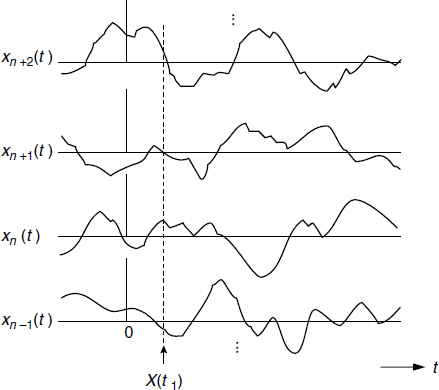
Figure 1.2 A few sample functions of a stochastic process
- A family (or ensemble) of time functions. Both t and s are variables.
- A single time function called a sample function or a realization of the stochastic process. Then t is a variable and s is fixed.
- A random variable; t is fixed and s is variable.
- A single number; both t and s are fixed.
Which of these four interpretations holds in a specific case should follow from the context.
Different classes of stochastic processes may be distinguished. They are classified on the basis of the characteristics of the realization values of the process x and the time parameter t. Both can be either continuous or discrete, in any combination. Based on this we have the following classes:
- Both the values of X(t) and the time parameter t are continuous. Such a process is called a continuous stochastic process.
- The values of X(t) are continuous, whereas time t is discrete. These processes are called discrete-time processes or continuous random sequences. In the remainder of the book we will use the term discrete-time process.
- If the values of X(t) are discrete but the time axis is continuous, we call the process a discrete stochastic process.
- Finally, if both the process values and the time scale are discrete, we say that the process is a discrete random sequence.
In Table 1.1 an overview of the different classes of processes is presented. In order to get some feeling for stochastic processes we will consider a few examples.
Table 1.1 Summary of names of different processes

1.3.1 Continuous Stochastic Processes
For this class of processes it is assumed that in principle the following holds:
![]()
An example of this class was already given by Figure 1.2. This could be an ensemble of realizations of a thermal noise process as is, for instance, produced by a resistor, the characteristics of which are to be dealt with in Chapter 6. The underlying experiment is selecting a specific resistor from a collection of, let us say, 100 Ω resistors. The voltage across every selected resistor corresponds to one of the realizations in the figure.
Another example is given below.
Example 1.1:
The process we consider now is described by the equation
![]()

Figure 1.3 Ensemble of sample functions of the stochastic process cos(ω0t − Θ), with Θ uniformly distributed on the interval (0, 2π]
with ω0 a constant and Θ a random variable with a uniform probability density function on the interval (0, 2π]. In this example the set of realizations is in fact uncountable, as Θ assumes continuous values. The ensemble of sample functions is depicted in Figure 1.3.
Thus each sample function consists of a cosine function with unity amplitude, but the phase of each sample function differs randomly from others. For each sample function a drawing is taken from the uniform phase distribution. We can imagine this process as follows. Consider a production process of crystal oscillators, all producing the same amplitude unity and the same radial frequency ω0. When all those oscillators are switched on, their phases will be mutually independent. The family of all measured output waveforms can be considered as the ensemble that has been presented in Figure 1.3.
This process will get further attention in different chapters that follow.
![]()
1.3.2 Discrete-Time Processes (Continuous Random Sequences)
The description of this class of processes becomes more and more important due to the increasing use of modern digital signal processors which offer flexibility and increasing speed and computing power. As an example of a discrete-time process we can imagine sampling the process that was given in Figure 1.2. Let us suppose that to this process ideal sampling is applied at equidistant points in time with sampling period Ts; with ideal sampling we mean the sampling method where the values at Ts are replaced by delta functions of amplitude X(nTs) [6]. However, to indicate that it is now a discrete-time process we denote it by X[n], where n is an integer running in principle from −∞ to +∞. We know from the sampling theorem (see Section 3.5.1 or, for instance, references [1] and [7]) that the original signal can perfectly be recovered from its samples, provided that the signals are band-limited. The process that is produced in this way is given in Figure 1.4, where the sample values are presented by means of the length of the arrows.

Figure 1.4 Example of a discrete-time stochastic process
Another important example of the discrete-time process is the so-called Poisson process, where there are no equidistant samples in time but the process produces ‘samples’ at random points in time. This process is an adequate model for shot noise and it is dealt with in Chapter 8.
1.3.3 Discrete Stochastic Processes
In this case the time is continuous and the values discrete. We present two examples of this class. The second one, the random data signal, is of great practical importance and we will consider it in further detail in Chapter 4.
Example 1.2:
This example is a very simple one. The ensemble of realizations consists of a set of constant time functions. According to the outcome of an experiment one of these constants may be chosen. This experiment can be, for example, the rolling of a die. In that case the number of realizations can be six (n = 6), equal to the usual number of faces of a die. Each of the outcomes s ∈ {1, 2, 3, 4, 5, 6} has a one-to-one correspondence to one of these numbered constant functions of time. The ensemble is depicted in Figure 1.5.
![]()
Example 1.3:
Another important stochastic process is the random data signal. It is a signal that is produced by many data sources and is described by
![]()
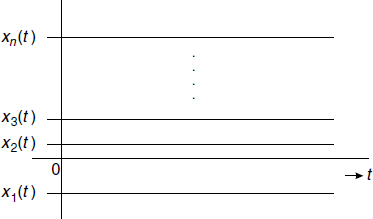
Figure 1.5 Ensemble of sample functions of the stochastic process constituted by a number of constant time functions
where {An} are the data bits that are randomly chosen from the set An ∈ {+1, −1}. The rectangular pulse p(t) of width T serves as the carrier of the information. Now Θ is supposed to be uniformly distributed on the bit interval (0, T], so that all data sources of the family have the same bit period, but these periods are not synchronized. The ensemble is given in Figure 1.6.
![]()
1.3.4 Discrete Random Sequences
The discrete random sequence can be imagined to result from sampling a discrete stochastic process. Figure 1.7 shows the result of sampling the random data signal from Example 1.3.
We will base the further development of the concept, description and properties of stochastic processes on the continuous stochastic process. Then we will show how these are extended to discrete-time processes. The two other classes do not get special attention, but are considered as special cases of the former ones by limiting the realization values x to a discrete set.

Figure 1.6 Ensemble of sample functions of the stochastic process Σn Anp(t − nT − Θ), with Θ uniformly distributed on the interval (0, T]

Figure 1.7 Example of a discrete random sequence
1.3.5 Deterministic Function versus Stochastic Process
The concept of the stochastic process does not conflict with the theory of deterministic functions. It should be recognized that a deterministic function can be considered as nothing else but a special case of a stochastic process. This is elucidated by considering Example 1.1. If the random variable Θ is given the probability density function fΘ(θ) = δ(θ), then the stochastic process reduces to the function cos(ω0t). The given probability density function is actually a discrete one with a single outcome. In fact, the ensemble of the process reduces in this case to a family comprising merely one member. This is a general rule; when the probability density function of the stochastic process that is governed by a single random variable consists of a single delta function, then a deterministic function results. This way of generalization avoids the often confusing discussion on the difference between a deterministic function on the one hand and a stochastic process on the other hand. In view of the consideration presented here they can actually be considered as members of the same class, namely the class of stochastic processes.
1.4 SUMMARY
Definitions of random signals and noise have been given. A random signal is, as a rule, an information carrying wanted signal that behaves randomly. Noise also behaves randomly but is unwanted and disturbs the signal. A common tool to describe both is the concept of a stochastic process. This concept has been explained and different classes of stochastic processes have been identified. They are distinguished by the behaviour of the time parameter and the values of the process. Both can either be continuous or discrete.
Introduction to Random Signals and Noise W. van Etten © 2005 John Wiley & Sons, Ltd