8

Poisson Processes and Shot Noise

8.1 INTRODUCTION

Random point processes described in this chapter deal with a sequences of events, where both the time and the amplitude of the random variable is of a discrete nature. However, in contrast to the discrete-time processes dealt with so far, the samples are not equidistant in time, but the randomness is in the arrival times. In addition, the sample values may also be random. In this chapter we will not deal with the general description of random point processes but will confine the discussion to a special case, namely those processes where the number of events k, in fixed time intervals of length T, is described by a Poisson probability distribution

In this equation we do not use the notation for the probability density function, since it is a discrete function and thus indeed a probability (denoted by P(·)) rather than a density, which is denoted by f_X(x).

An integer-valued stochastic process is called a Poisson process if the following properties hold [1,5]:

1. The probability that k events occur in any arbitrary interval of length T is given by Equation (8.1).
2. The number of events that occur in any arbitrary time interval is independent of the number of events that occur in any other arbitrary non-overlapping time interval.

Many physical phenomena are accurately modelled by a Poisson process, such as the emission of photons from a laser source, the generation of hole/electron pairs in photodiodes by means of photons, the arrival of phone calls in an exchange, the number of jobs offered to a processor and the emission of electrons from a cathode.

In this chapter we will deal with the most important parameters of both Poisson processes with a constant expectation, called homogeneous Poisson processes, and processes with an expectation that is a function of time, called inhomogeneous Poisson processes. In both models, the amplitude of the physical phenomenon that is related to the events is constant, for instance the arrival of phone calls one at a time. Moreover, we will develop some theory about stochastic processes, as far as it relates to Poisson processes. Finally, we will consider Poisson impulse processes; these are processes where the amplitude of the event is a random variable as well. An example of such a process is the number of electrons produced in a photomultiplier tube, where the primary electrons (electrons that are directly generated by photon absorption) are subject to a random gain. A similar effect occurs in an avalanche photodiode [8].

8.2 THE POISSON DISTRIBUTION

8.2.1 The Characteristic Function

When dealing with Poisson and related processes, it appears that the characteristic function is a convenient tool to use in the calculation of important properties of the process, such as mean value, variance, etc.; this will become clear later on. The characteristic function of a random variable X is defined as

where f_X(x) is the probability density function of X. Note that according to this definition the characteristic function is closely related to the Fourier transform of the probability density function, namely Φ(−u) is the Fourier transform of f_X(x). The variable u is just a dummy variable and has no physical meaning. When X is a discrete variable with the possible realizations {X_k}, then the definition becomes

Sometimes it is useful to consider the logarithm of the characteristic function

This function is called the second characteristic function of the random variable X. From Equation (8.2) it follows that

so that

For the random variable Y = aX + b, with a and b as constants, it follows that

and

When on the other hand the characteristic function is known, the probability density function can be restored from it using the inverse Fourier integral transform

The next example shows that defining the characteristic function by means of the Fourier transform of the probability density function is a powerful tool and can greatly simplify certain calculations.

The moments of the random variable X are defined by

It follows, using Fourier transform theory, that a relationship between the derivatives of the characteristic function and these moments can be established. This relationship is found by expanding the exponential of the integrand of Equation (8.2) as follows:

Assuming that integration term by term is allowed, it follows that

From this equation the moments can immediately be identified as

The operations leading to Equation (8.16) are allowed if all the moments m_n exist and the series expansion of Equation (8.15) converges absolutely at u = 0. In this case f_X(x) is uniquely determined by its moments m_n.

Sometimes it is more interesting to consider the central moments, e.g. the second central moment or variance. Then the preceding operations are applied to the random variable X − E[X], but for such an important central moment as the variance there is an alternative, as will be shown in the sequel.

8.2.2 Cumulants

Consider a probability distribution of which all the moments of arbitrary order exist. In the characteristic function ju is replaced by p and the function that results is called the moment generating function. The logarithm of this function becomes

Now, expanding Ψ(p) into a Taylor series about p = 0 and remembering that

it is found that

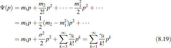
where σ² is the variance of X and γ_k is the kth cumulant or semi-invariant [1,15].

8.2.3 Interarrival Time and Waiting Time

For such problems as queuing, it is of importance to know the probability density function of the time that elapses between two events; this time is called the interarrival time. Suppose that an event took place at time t; then the probability that the random waiting time W is greater than some fixed value w represents the probability that no event occurs in the time interval {t, t + w}, or

and

Thus, the waiting time is an exponential random variable and its probability density function is written as

The mean waiting time has the value

This result can also easily be understood when remembering that λ is the mean number of events per unit of time. Then the mean waiting time will be its inverse.

8.3 THE HOMOGENEOUS POISSON PROCESS

Let us consider an homogeneous Poisson process defined as the sum of impulses

where the δ impulses δ(t − t_i) appear at random times {t_i} governed by a Poisson distribution. This process can be used for modelling such physical processes as the detection of photons by a photodetector. Each time an arriving photon is detected, it causes a small impulse-shaped amount of current having an amplitude equal to the charge of an electron. This means that the photon arrival and thus the production of current impulses may be described by Equation (8.25), depicted as the input of Figure 8.1(b). Due to the travel time of the moving charges in the detector and the frequency-dependent load circuit (see Figure 8.1(a)), the response of the current through the load will have a different shape, for instance as given in Figure 8.1(b). The shape of this response is called h(t), being the impulse response of the circuit. The total voltage across the load is described by the process

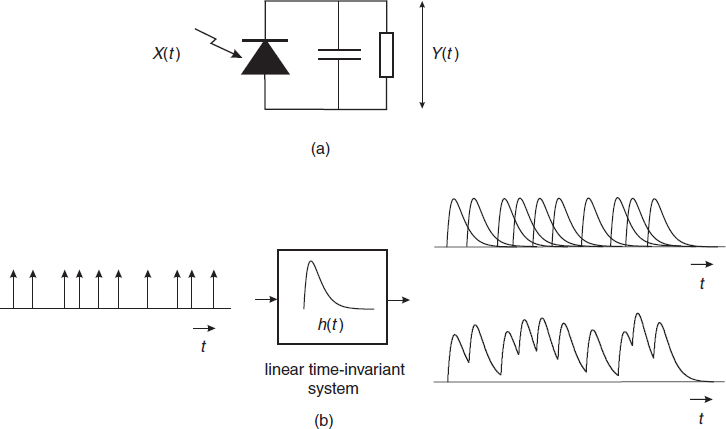
Figure 8.1 (a) Photodetector circuit with load and (b) corresponding Poisson process and shot noise process

This process is called shot noise and even if the rate λ of the process is constant (in the example of the photodetector the constant amount of optical power arriving), the process Y(t) will indeed show a noisy character, as has been depicted in the output of Figure 8.1(b). The upper curve at the output represents the individual responses, while the lower curve shows the sum of these pulses. Calculating the probability density function of this process is a difficult problem, but we will be able to calculate its mean value and autocorrelation function, and thus its spectrum as well.

8.3.1 Filtering of Homogeneous Poisson Processes and Shot Noise

In order to simplify the calculation of the mean value and the autocorrelation function of the shot noise, the time axis is subdivided into a sequence of consecutive small time intervals of equal width Δt. These time intervals are taken so short that λΔt 1. Next we define the random variable V_n such that for all integer values n

In the sequel we shall neglect the probability that more than one impulse will occur in such a brief time interval as Δt. Following the definition of a Poisson process as given in the introduction to this chapter, it is concluded that the random variables V_n and V_m are independent if n ≠ m. The probabilities of the two possible realizations of V_n read

where the exact expressions are achieved by inserting k = 0 and k = 1, respectively, in Equation (8.1) and the approximations follow from the fact that λΔt 1. The expectation of the random variable V_n is

Based on the foregoing it is easily revealed that the process Y(t) is approximated by the process

The smaller the Δt the closer the approximation (t) will approach the shot noise process Y(t); in the limit of Δt approaching zero, the processes will merge. The expectation of (t) is

When Δt is made infinitesimally small then the summation is converted into an integral and the expected value of the shot noise process is obtained:

In order to gain more information about the shot noise process we will consider its characteristic function. This function is deduced in a straightforward way using the approximation (t):

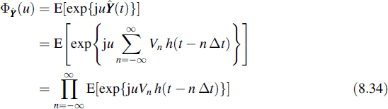
In Equation (8.34) the change from the summation in the exponential to the product of the expectation of the exponentials is allowed since the random variables V_n are independent. Invoking the law of total probability, the characteristic function of (t) is written as

and using Equations (8.28) and (8.29) gives

Now we use the approximation 1 + x ≈ exp(x) to proceed as

Once again Δt is made infinitesimally small so that the summation converts into an integral and we arrive at the characteristic function of the shot noise process Y(t):

From this result several features of the shot noise can be deduced. By inverse Fourier transforming it, we find the probability density function of Y(t), but this is in general a difficult task. However, the mean and variance of the shot noise process follow immediately from the second characteristic function

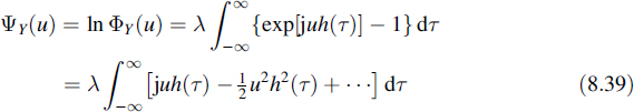
and by invoking Equation (8.19).

Actually, the result of Equation (8.40) was earlier derived in Equation (8.33), but here we found this result in an alternative way. We emphasize that both the mean value and variance are proportional to the Poisson parameter λ. When the mean value of the shot noise process is interpreted as the signal and the variance as the noise, then it is concluded that this type of noise is not additive, as in the classical communication model, but multiplicative; i.e. the noise variance is proportional to the signal value and the signal-to-shot noise ratio is proportional to λ.

Next we want to calculate the autocorrelation function R_Y(t₁, t₂) of the shot noise process and from that the power spectrum. For that purpose we define the joint characteristic function of two random variables X₁ and X₂ as

Actually, this function is the two-dimensional Fourier transform of the joint probability density function of X₁ and X₂. In order to evaluate this function for the shot noise process Y(t) we follow a similar procedure as before, i.e. we start with the approximating process (t):

Elaborating this in a straightforward manner as before (see Equations (8.34) to (8.38)) we arrive at the joint characteristic function of Y(t):

The second joint characteristic function reads

In the sequel we shall show that by series expansion of this latter function, the autocorrelation function can be calculated. However, we will first show how moments of several orders are generated by the joint characteristic function. For that purpose we apply series expansion to both exponentials in Equation (8.44):

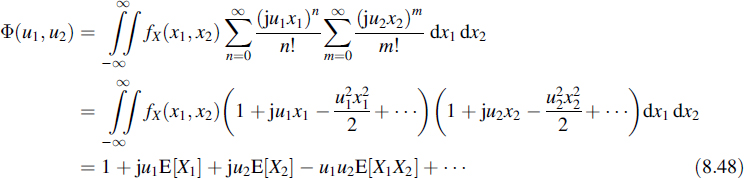
From this equation it is observed that the term with ju₁ comprises E[X₁], the term with ju₂ comprises E[X₂], the term with −u₁u₂ comprises E[X₁X₂], etc. In fact, series expansion of the joint characteristic function generates all arbitrary moments as follows:

Since the characteristic function given by Equation (8.46) contains a double exponential, producing a series expansion is intractable. Therefore we make a series expansion of the second joint characteristic function of Equation (8.47) and identify from that expansion the second-order moment E[Y(t₁)Y(t₂)] we are looking for. This expansion is once again based on the series expansion of the logarithm ln(1 + x) = x − x²/2 + …:

When looking at the term with u₁u₂, we discover that its coefficient reads −(E[X₁X₂]−E[X₁]E[X₂]). Comparing this expression with Equation (2.65) and applying it to the process Y(t) it is revealed that this coefficient equals the negative of the autocovariance function C_YY(t₁, t₂). As we have already calculated the mean value of the process (see Equations (8.33) and (8.40)), we can easily obtain its autocorrelation function. To evaluate this function we expand Equation (8.47) in a similar way and look for the coefficient of the term with u₁u₂. This yields

We observe that this expression does not depend on the absolute time, but only on the difference t₂ − t₁. Since the mean was independent of time as well, it is concluded that the shot noise process is wide-sense stationary. Its autocorrelation function reads

From this we can immediately find the power spectrum by Fourier transforming the latter expression:

It can be seen that the spectrum always comprises a d.c. component if this component is passed by the filter, i.e. if H(0) ≠ 0. As a special case we consider the spectrum of the input process X(t) that consists of a sequence of Poisson impulses as given by Equation (8.25). This spectrum is easily found by inserting H(ω) = 1 in Equation (8.53). Then, apart from the δ function, the spectrum comprises a constant value, so this part of the spectrum behaves as white noise.

For large values of the Poisson parameter λ, the shot noise process approaches a Gaussian process [1]. This model is widely used for the shot noise generated by electronic components.

8.4 INHOMOGENEOUS POISSON PROCESSES

An inhomogeneous Poisson process is a Poisson process for which the parameter λ varies with time, i.e. λ = λ(t). In order to derive the important properties of such a process we redo the calculations of the preceding section, where the parameter λ in Equations (8.28) to (8.37) is replaced by λ(n Δt). The characteristic function then becomes

Based on Equation (8.19), the mean and variance of this process follows immediately:

Actually, these two equations are an extension of Campbell's theorem.

Without going into detail, the autocorrelation function of this process is easily found in a way similar to the procedure of calculating the second joint characteristic function in the preceding section. The second joint characteristic function of the inhomogeneous Poisson process is obtained as

and from this, once again, similarly to the preceding section, it follows that

Let us now suppose that the function λ(t) is a stochastic process as well, which is independent of the Poisson process. Then the process Y(t) is a doubly stochastic process [17]. Moreover, we assume that λ(t) is a wide-sense stationary process. Then from Equation (8.55) it follows that the mean value of Y(t) is independent of time. In the autocorrelation function we substitute t₁ = t and t₂ = t + τ; this yields

In this equation R_λλ(·) is the autocorrelation function of the process λ(t). Further elaborating the Equation (8.59) gives

Now it is concluded that the doubly stochastic process Y(t) is wide-sense stationary as well. From this latter expression its power spectral density is easily revealed by Fourier transformation:

The interpretation of this expression is as follows. The first term reflects the filtering of the white shot noise spectrum and is proportional to the mean value of the information signal λ(t). Note that E[λ(t)] = 0 is meaningless from a physical point of view. The second term represents the filtering of the information signal.

An important physical situation where the theory in this section applies is a lightwave that is intensity modulated by an information signal. The detected current in the receiver is produced by photons arriving in the photodetector. This arrival of photons is then modelled as a doubly stochastic process with λ(t) as the information signal [8].

8.5 THE RANDOM-PULSE PROCESS

Let us further extend the inhomogeneous process that was introduced in the preceding section. A Poisson impulse process consists of a sequence of δ functions

where the number of events per unit of time are governed by a Poisson distribution and {G_i} are realizations of the random variable G; i.e. the amplitudes of the different impulses vary randomly and thus are subject to a random gain. In this section we again assume that the Poisson distribution may have a time-variant parameter λ(t), which is supposed to be a wide-sense stationary stochastic process. Each of three random parameters involved is assumed to be independent of all the others. When filtering the process X(t) we get the random-pulse process

The properties of this process are again derived in a similar and straightforward way, as presented in Section 8.3.1. Throughout the entire derivation a third random variable is involved and the expectation over this variable has to be taken in addition. This leads to the following result for the characteristic function:

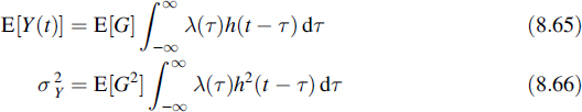
where Φ_G(u) is the characteristic function of G. From this another extension of Campbell's theorem follows:

The second joint characteristic function reads

where f_G(g) is the probability density function of G. Also in this case the process Y(t) appears to be wide-sense stationary and the autocorrelation function becomes

and the power spectral density

The last term will in general comprise the information, whereas the first term is the shot noise spectral density. In applications where the random impulse amplitude G is an amplification generated by an optical or electronic device, the factor E[G²]/E²[G] is called the excess noise factor. It is the factor by which the signal-to-shot noise ratio is decreased compared to the situation where such amplification is absent, i.e. G is constant and equal to 1. Since

the excess noise factor is always larger than 1.

There are two main application areas for the processes dealt with in this section. The first example is the current produced by a photomultiplier tube or avalanche photodiode when an optical signal is detected. Each detected photon produces many electrons as a consequence of the internal amplification in the detector device. This process can be modelled as a Poisson impulse process, where G is a random variable with discrete integer amplitude. Looking at Equation (8.70) one may wonder why such amplification is applied when the signal-to-noise ratio is decreased by it. From the first line in this equation it is revealed that the information signal is amplified by E²[G] and that is useful, since it raises the signal level with respect to the thermal noise (not taken into account in this chapter), which is dominant over the shot noise in the case of weak signal reception.

Secondly, when a radar on board an aircraft flying over the sea transmits pulses, it receives many copies of the transmitted pulse, called clutter. These echoes are randomly distributed in time and amplitude, due to reflections from the moving water waves. Similar reflections are received when flying over land, due to the relative changes in the earth's surface and eventual buildings. This process may be modelled as a random-pulse process.

8.6 SUMMARY

The Poisson distribution is recalled. Subsequently, the characteristic function is defined. This function provides a powerful tool for calculating moments of random variables. When taking the logarithm of the characteristic function, the second characteristic function results and it can be of help calculating moments of Poisson distributions and processes. Based on these functions several properties of the Poisson distribution are derived. The probability density function of the interarrival time is calculated.

The homogeneous Poisson process consists of a sequence of unit impulses with random distribution on the time axis and a Poisson distribution of the number of impulses per unit of time. When filtering this process a noise-like signal results, called shot noise. Based on the characteristic function and the second characteristic function several properties of this process are derived, such as the mean value, variance (Campbell's theorem) and autocorrelation function. From these calculations it follows that the homogeneous Poisson process is a wide-sense stationary process. Fourier transforming the autocorrelation function provides the power spectral density. Although part of the shot noise process behaves like white noise, it is not additive but multiplicative. Derivation of the properties of the inhomogeneous Poisson process and the random-pulse process is similar to that of the homogeneous Poisson process.

Although our approach emphasizes using the characteristic function to calculate the properties of random point processes, it should be stressed that this is not the only way to arrive at these results. A few application areas of random point processes are mentioned.

8.7 PROBLEMS

8.1 Consider two independent random variables X and Y. The random variable Z is defined as the sum Z = X + Y. Based on the use of characteristic functions show that the probability density function of Z equals the convolution of the probability density functions of X and Y.

8.2 Calculate the characteristic function of a Gaussian random variable.

8.3 Consider two jointly Gaussian random variables, X and Y, both having zero mean and variance of unity. Using the characteristic functions show that the probability density function of their sum, Z = X + Y, is Gaussian as well.

8.4 Use the characteristic function to calculate the variance of the waiting time of a Poisson process.

8.5 The characteristic function can be used to calculate the probability density function of a function g(X) of a random variable if the transformation Y = g(X) is one-to-one. Consider Y = sin X, where X is uniformly distributed on the interval (−π/2, π/2].

(a) Calculate the probability density function of Y.

(b) Use the result of (a) to calculate the probability density function of a full sine wave, i.e. Y = sin X, where now X is uniformly distributed on the interval (−π, π] Hint: extend the sine wave so that X uniformly covers the interval (−π, π].

8.6 A circuit comprises 100 components. The circuit fails if one of the components fails. The time to failure of one component is exponentially distributed with a mean time to failure of 10 years. This distribution is the same for all components and the failure of each components is independent of the others.

(a) What is the probability that the circuit will be in operation for at least one year without interruption due to failure?

(b) What should the mean time to failure of a single component be so that the probability that the circuit will be in operation for at least one year without interruption is 0.9?

8.7 A switching centre has 100 incoming lines and one outgoing line. The arrival of calls is Poisson distributed with an average rate of 5 calls per hour. Suppose that each call lasts exactly 3 minutes.

(a) Calculate the probability that an incoming call finds the outgoing line blocked.

(b) The subscribers have a contract that guarantees a blocking probability less than 0.01. They complain that the blocking probability is higher than what was promised in the contract with the provider. Are they right?

(c) How many outgoing lines are needed to meet this condition in the contract?

8.8 Visitors enter a museum according to a Poisson distribution with a mean of 10 visitors per hour. Each visitor stays in the museum for exactly 0.5 hour.

(a) What is the mean value of the number of visitors present in the museum?

(b) What is the variance of the number of visitors present in the museum?

(c) What is the probability that there are no visitors in the museum?

8.9 Consider a shot noise process with constant parameter λ. This process is applied to a filter that has the impulse response h(t) = exp(−αt) u(t), with u(t) the unit step function.

(a) Find the mean value of the filtered shot noise process.

(b) Find the variance of the filtered process.

(c) Find the autocorrelation function of the filtered process.

(d) Calculate the power spectral density of the filtered process.

8.10 We want to consider the properties of a filtered shot noise process Y(t) with constant parameter λ 1. The problem is that when λ → ∞ both the mean and the variance become infinitely large. Therefore we consider the normalized process with zero mean and variance of unity for all λ values:

where

Apply Equation (8.38) and the series expansion of Equation (8.39) to the process Ξ(t) to prove that the characteristic function of Ξ(t) tends to that of a Gaussian random variable (see the outcome of Problem 8.2) and thus the filtered Poisson process approaches a Gaussian process when the Poisson parameter λ becomes large.

8.11 The amplitudes of the impulses of a Poisson impulse process are independent and identically distributed with P(G_i = 1) = 0.6 and P(G_i = 2) = 0.4. The process is applied to a linear time-invariant filter with a rectangular impulse response of height 10 and duration T. The Poisson parameter λ is constant.

(a) Find the mean value of the filter output process.

(b) Find the autocorrelation function of the filter output process.

(c) Calculate the power spectral density of the output process.

8.12 The generation of hole-electron pairs in a photodiode is modelled as a Poisson process due to the random arrival of photons. When the optical wave is modulated by a randomly phased harmonic signal this arrival has a time-dependent rate of

with Θ a random variable that is uniformly distributed on the interval (0, 2π], and where the cosine term is the information-carrying signal. Each hole-electron pair creates an impulse of height e, being the electron charge. The photodetector has a random internal gain that has only integer values and that is uniformly distributed on the interval [0, 10]. The travel time T in the detector is modelled as an impulse response

(a) Calculate the mean value of the photodiode current and the power of the detected signal current.

(b) Calculate the shot noise variance.

(c) Calculate the the signal-to-noise ratio in dB for λ₀ = 7.5 × 10¹², T = 10⁻⁹ and ω₀ = 2π × 0.5 × 10⁹.