
7
Detection and Optimal Filtering
Thus far the treatment has focused on the description of random signals and their analyses, and how these signals are transformed by linear time-invariant systems. In this chapter we take a somewhat different approach; namely starting with what is known about input processes and of system requirements we look for an optimum system. This means that we are going to perform system synthesis. The approach achieves an optimal reception of information signals that are corrupted by noise. In this case the input process consists of two parts, the information bearing or data signal and noise, and we may wonder what the optimal receiver or processing looks like, subject to some criterion.
When designing an optimal system three items play a crucial role. These are:
- A description of the input noise process and the information bearing signal;
- Conditions to be imposed on the system;
- A criterion that defines optimality.
In the following we briefly comment on these items:
- It is important to know the properties of the system inputs, e.g. the power spectral density of the input noise, whether it is wide-sense stationary, etc. What does the information signal look like? Are information signal and noise additive or not?
- The conditions to be imposed on the system may influence performance of the receiver or the processing. We may require the system to be linear, time-invariant, realizable, etc. To start with and to simplify matters we will not bother about realizability. In specific cases it can easily be included.
- The criterion will depend on the problem at hand. In the first instance we will consider two different criteria, namely the minimum probability of error in detecting data signals and the maximum signal-to-noise ratio. These criteria lead to an optimal linear filter called the matched filter. This name will become clear in the sequel. Although the criteria are quite different, we will show that there is a certain relationship in specific cases. In a third approach we will look for a filter that produces an optimum estimate of the realization of a stochastic process, which comes along with additive noise. In such a case we use the minimum mean-squared error criterion and end up with the so-called Wiener filter.
7.1 SIGNAL DETECTION
7.1.1 Binary Signals in Noise
Let us consider the transmission of a known deterministic signal that is disturbed by noise; the noise is assumed to be additive. This situation occurs in a digital communication system where, during successive intervals of duration T seconds, a pulse of known shape may arrive at the receiver (see the random data signal in Section 4.5). In such an interval the pulse has been sent or not. In accordance with Section 4.5 this transmitted random data signal is denoted by
Here An is randomly chosen from the set {0, 1}. The received signal is disturbed by additive noise. The presence of the pulse corresponds to the transmission of a binary digit ‘1’ (An = 1), whereas absence of the pulse in a specific interval represents the transmission of a binary digit ‘0’ (An = 0). The noise is assumed to be stationary and may originate from disturbance of the channel or has been produced in the front end of the receiver equipment. Every T seconds the receiver has to decide whether a binary ‘1’ or a binary ‘0’ has been sent. This decision process is called detection. Noise hampers detection and causes errors to occur in the detection process, i.e. ‘1’s may be interpreted as ‘0’s and vice versa.
During each bit interval there are two possible mutually exclusive situations, called hypotheses, with respect to the received signal R(t):

The hypothesis H0 corresponds to the situation that a ‘0’ has been sent (An = 0). In this case the received signal consists only of the noise process N(t). Hypothesis H1 corresponds to the event that a ‘1’ has been sent (An = 1). Now the received signal comprises the known pulse shape p(t) and the additive noise process N(t). It is assumed that each bit occupies the (0, T) interval. Our goal is to design the receiver such that in the detection process the probability of making wrong decisions is minimized. If the receiver decides in favour of hypothesis H0 and it produces a ‘0’, we denote the estimate of An by Ân and say that Ân = 0. In case the receiver decides in favour of hypothesis H1 and a ‘1’ is produced, we denote Ân = 1. Thus the detected bit Ân ∈ {0, 1}. In the detection process two types of errors can be made. Firstly, the receiver decides in favour of hypothesis H1, i.e. a ‘1’ is detected (Ân = 1), whereas a ‘0’ has been sent (An = 0). The conditional probability of this event is P(Ân = 1 | H0) = P(Ân = 1 | An = 0). Secondly, the receiver decides in favour of hypothesis H0 (Ân = 0), whereas a ‘1’ has been sent (An = 1). The conditional probability of this event is P(Ân = 0 | H1) = P(Ân = 0 | An = 1). In a long sequence of transmitted bits the prior probability of sending a ‘0’ is given by P0 and the prior probability of a ‘1’ by P1. We assume that these probabilities are known in the receiver. In accordance with the law of total probability the bit error probability is given by

This error probability is minimized if the receiver chooses the hypothesis with the highest conditional probability, given the process R(t). It will be clear that the conditional probabilities of Equation (7.4) depend on the signal p(t), the statistical properties of the noise N(t) and the way the receiver processes the received signal R(t). As far as the latter is concerned, we assume that the receiver converts the received signal R(t) into K numbers (random variables), which are denoted by the K-dimensional random vector
The receiver chooses the hypothesis H1 if P(H1 | r) ≥ P(H0 | r), or equivalently P1 fr(r | H1) ≥ P0 fr(r | H0), since it follows from Bayes' theorem (reference [14]) that
From this it follows that the decision can be based on the so-called likelihood ratio
In other words, hypothesis H1 is chosen if Λ(r) > Λ0 and hypothesis H0 is chosen if Λ(r) < Λ0. The quantity Λ0 is called the decision threshold. In taking the decision the receiver partitions the vector space spanned by r into two parts, R0 and R1, called the decision regions. The boundary between these two regions is determined by Λ0. In the region R0 we have the relation Λ(r) < Λ0 and an observation of r in this region causes the receiver to decide that a binary ‘0’ has been sent. An observation in the region R1, i.e. Λ(r) ≥ Λ0, makes the receiver decide that a binary ‘1’ has been sent. The task of the receiver therefore is to transform the received signal R(t) into the random vector r and determine to which of the regions R0 or R1 it belongs. Later we will go into more detail of this signal processing.
Example 7.1:
Consider the two conditional probability densities

![]()
and the prior probabilities

Figure 7.1 Conditional probability density functions of the example and the decision regions R0 and R1
Let us calculate the decision regions for this situation. By virtue of Equation (7.10) the decision threshold is set to one and the decision regions are found by equating the right-hand sides of Equations (7.8) and (7.9):

The two expressions are depicted in Figure 7.1. As seen from the figure, the functions are even symmetric and, confining to positive values of r, this equation can be rewritten as the quadratic
Solving this yields the roots r1 = 0.259 and r2 = 1.741. Considering negative r values produces the same negative values for the roots. Hence it may be concluded that the decision regions are described by

![]()
One may wonder what to do when an observation is exactly at the boundaries of the decision regions. An arbitrary decision can be made, since the probability of this event approaches zero.
The conditional error probabilities in Equation (7.4) are written as

The minimum total bit error probability is found by inserting these quantities in Equation (7.4).
Example 7.2:
An example of a received data signal (see Equation (7.1)) has been depicted in Figure 7.2(a). Let us assume that the signal R(t) is characterized by a single number r instead of a vector and that in the absence of noise (N(t) ≡ 0) this number is symbolically denoted by ‘0’ (in the case of hypothesis H0) or ‘1’ (in the case of hypothesis H1). Furthermore, assume that in the presence of noise N(t) a stochastic Gaussian variable should be added to this characteristic number. For this situation the conditional probability density functions are given in Figure 7.2(a) upper right. In Figure 7.2(b) these functions are depicted once more, but now in a somewhat different way. The boundary that separates the decision regions R0 and R1 reduces to a single point. This point r0 is determined by Λ0. The bit error probability is now written as

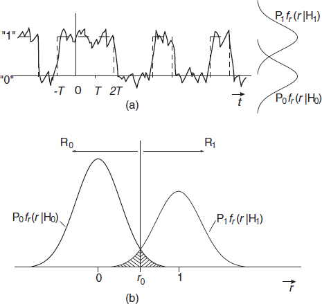
Figure 7.2 (a) A data signal disturbed by Gaussain noise and (b) the corresponding weighted (by the prior probabilities) conditional probability density functions and the decision regions R0 and R1
The first term on the right-hand side of this equation is represented by the right shaded region in Figure 7.2(b) and the second term by the left shaded region in this figure. The threshold value r0 is to be determined such that Pe is minimized. To that end Pe is differentiated with respect to r0
When this expression is set equal to zero we once again arrive at Equation (7.7); in this way this equation has been deduced in an alternative manner. Now it appears that the optimum threshold value r0 is found at the intersection point of the curves P0 fr(r | H0) and P1 fr (r | H1). If the probabilities P0 and P1 change but the probability density function of the noise N(t) remains the same, then the optimum threshold value shifts in the direction of the binary level that corresponds to the shrinking prior probability.
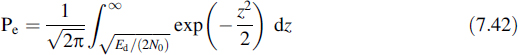
Remembering that we considered the case of Gaussian noise, it is concluded that the integrals in Equation (7.17) can be expressed using the well-known Q function (see Appendix F), which is defined as

This function is related to the erfc(·) function as follows:
Both functions are tabulated in many books or can be evaluated using software packages. They are presented graphically in Appendix F.
More details on the Gaussian noise case are presented in the next section.
![]()
7.1.2 Detection of Binary Signals in White Gaussian Noise
In this subsection we will assume that in the detection process as described in the foregoing the disturbing noise N(t) has a Gaussian probability density function and a white spectrum with a spectral density of N0/2. This latter assumption means that filtering has to be performed in the receiver. This is understood if we realize that a white spectrum implies an infinitely large noise variance, which leads to problems in the integrals that appear in Equation (7.17). Filtering limits the extent of the noise spectrum to a finite frequency band, thereby limiting the noise variance to finite values and thus making the integrals well defined.
The received signal R(t) is processed in the receiver to produce the vector r in a signal space {φk(t)} that completely describes the signal p(t) and is assumed to be an orthonormal set (see Appendix A)

As the operation given by Equation (7.21) is a linear one, it can be applied to the two terms of Equation (7.3) separately, so that
with

and

In fact, the processing in the receiver converts the received signal R(t) into a vector r that consists of the sum of the deterministic signal vector p, of which the elements are given by Equation (7.23), and the noise vector n, of which the elements are given by Equation (7.24). As N(t) has been assumed to be Gaussian, the random variables nk will be Gaussian as well. This is due to the fact that when a linear operation is performed on a Gaussian variable the Gaussian character of the random variable is maintained. It follows from Appendix A that the elements of the noise vector are orthogonal and all of them have the same variance N0/2. In fact, the noise vector n defines the relevant noise (Appendix A and reference [14]).
Considering the case of binary detection, the conditional probability density functions for the two hypotheses are now

and

Using Equation (7.7), the likelihood ratio is written as

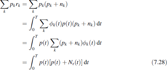
In Appendix A it is shown that the term ![]() represents the energy Ep of the deterministic signal p(t). This quantity is supposed to be known at the receiver, so that the only quantity that depends on the transmitted signal consists of the summation over pkrk. By means of signal processing on the received signal R(t), the value of this latter summation should be determined. This result represents a sufficient statistic [3,9] for detecting the transmitted data in an optimal way. A statistic is an operation on an observation, which is presented by a function or functional. A statistic is said to be sufficient if it preserves all information that is relevant for estimating the data. In this case it means that in dealing with the noise component of r the irrelevant noise components may be ignored (see Appendix A or reference [14]). This is shown as follows:
represents the energy Ep of the deterministic signal p(t). This quantity is supposed to be known at the receiver, so that the only quantity that depends on the transmitted signal consists of the summation over pkrk. By means of signal processing on the received signal R(t), the value of this latter summation should be determined. This result represents a sufficient statistic [3,9] for detecting the transmitted data in an optimal way. A statistic is an operation on an observation, which is presented by a function or functional. A statistic is said to be sufficient if it preserves all information that is relevant for estimating the data. In this case it means that in dealing with the noise component of r the irrelevant noise components may be ignored (see Appendix A or reference [14]). This is shown as follows:
where Nr(t) is the relevant noise part of N(t) (see Appendix A or reference [14]). Since the irrelevant part of the noise Ni(t) is orthogonal to the signal space (see Appendix A), adding this part of the noise to the relevant noise in the latter expression does not influence the result of the integration:

The implementation of this operation is as follows. The received signal R(t) is applied to a linear, time-invariant filter with the impulse response p(T − t). The output of this filter is sampled at the end of the bit interval (at t0 = T), and this sample value yields the statistic of Equation (7.29). This is a simple consequence of the convolution integral. The output signal of the filter is denoted by Y(t), so that

At the sampling instant t0 = T the value of the signal at the output is

The detection process proceeds as indicated in Section 7.1.1; i.e. the sample value Y(T) is compared to the threshold value. This threshold value D is found from Equations (7.27) and (7.7), and is implicitly determined by

Figure 7.3 Optimal detector for binary signals
Hypothesis H0 is chosen whenever Y(T) < D, whereas H1 is chosen whenever Y(T) ≥ D. In the special binary case where ![]() , it follows that D = Ep/2. Note that in the case at hand the signal space will be one-dimensional.
, it follows that D = Ep/2. Note that in the case at hand the signal space will be one-dimensional.
The filter with the impulse response h(t) = p(T − t) is called a matched filter, since the shape of its impulse response is matched to the pulse p(t). The scheme of the detector is very simple; namely the signal is filtered by the matched filter and the output of this filter is sampled at the instant t0 = T. If the sampled value is smaller than D then the detected bit is Ân = 0(H0) and if the sampled value is larger than D then the receiver decides Ân = 1(H1). This is represented schematically in Figure 7.3.
7.1.3 Detection of M-ary Signals in White Gaussian Noise
The situation of M-ary transmission is a generalization of the binary case. Instead of two different hypotheses and corresponding signals there are M different hypotheses, defined as

As an example of this situation we mention FSK; in binary FSK we have M = 2.
To deal with the M-ary detection problem we do not use the likelihood ratio directly; in order to choose the maximum likely hypothesis we take a different approach. We turn to our fundamental criterion; namely the detector chooses the hypothesis that is most probable, given the received signal. The probabilities of the different hypotheses, given the received signal, are given by Equation (7.6). When selecting the hypothesis with the highest probability, the denominator fr(r) may be ignored since it is common for all hypotheses. We are therefore looking for the hypothesis Hi, for which Pi fr(r | Hi) attains a maximum.
For a Gaussian noise probability density function this latter quantity is
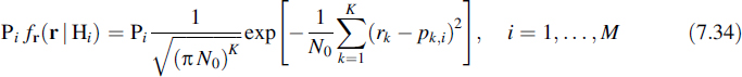
with pk,i the kth element of pi(t) in the signal space; the summation over k actually represents the distance in signal space between the received signal and pi(t) and is called the distance metric. Since Equation (7.34) is a monotone-increasing function of r, the decision may also be based on the selection of the largest value of the logarithm of expression (7.34). This means that we compare the different values of

The second and fifth term on the right-hand side are common for all hypotheses, i.e. they do not depend on i, and thus they may be ignored in the decision process. We finally end up with the decision statistics
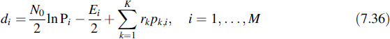
where Ei is the energy in the signal pi(t) (see Appendix A) and Equation (7.35) has been multiplied by N0/2, which is allowed since it is a constant and does not influence the decision. For ease of notation we define
so that
Based on Equations (7.37) and (7.38) we can construct the optimum detector. It is shown in Figure 7.4. The received signal is filtered by a bank of matched filters, the ith filter being matched to the signal pi(t). The outputs of the filters are sampled and the result represents the last term of Equation (7.38). Next, the bias terms bi given by Equation (7.37) are added to these outputs, as indicated in the figure. The resulting values di are applied to a circuit that selects the largest, thereby producing the detected symbol Â. This symbol is taken from the alphabet {A1, …, AM}, the same set of symbols from which the transmitter selected its symbols.

Figure 7.4 Optimal detector for M-ary signals where the symbols are mapped to different signals

Figure 7.5 Conditional probability density functions in the binary case with the error probability indicated by the shaded area
In all these operations it is assumed that the shapes of the several signals pi(t) as well as their energy contents are known and fixed, and the prior probabilities Pi are known. It is evident that the bias terms may be omitted in case all prior probabilities are the same and all signals pi(t) carry the same energy.
Example 7.3:
As an example let us consider the detection of linearly independent binary signals p0(t) and p1(t) in white Gaussian noise. The signal space to describe this signal set is two-dimensional. However, it can be reduced to a one-dimensional signal space by converting to a simplex signal set (see Section A.5). The basis of this signal space is given by ![]() where Ed is the energy in the difference signal. The signal constellation is given by the coordinates
where Ed is the energy in the difference signal. The signal constellation is given by the coordinates ![]() and
and ![]() and the distance between the signals amounts to
and the distance between the signals amounts to ![]() . Superimposed on these signals is the noise with variance N0/2 (see Appendix A, Equation (A.26)). We assume that the two hypotheses are equiprobable. The situation has been depicted in Figure 7.5. In this figure the two conditional probability density functions are presented. The error probability follows from Equation (7.17), and since the prior probabilities are equal we can conclude that
. Superimposed on these signals is the noise with variance N0/2 (see Appendix A, Equation (A.26)). We assume that the two hypotheses are equiprobable. The situation has been depicted in Figure 7.5. In this figure the two conditional probability density functions are presented. The error probability follows from Equation (7.17), and since the prior probabilities are equal we can conclude that
In the figure the value of the error probability is indicated by the shaded area. Since the noise has been assumed to be Gaussian, this probability is written as

Introducing the change of integration variable

the error probability is written as
This expression is recognized as the well-known Q function (see Equation (7.19) and Appendix F). Finally, the error probability can be denoted as
This is a rather general result that can be used for different binary transmission schemes, both for baseband and modulated signal formats. The conditions are that the noise is white, additive and Gaussian, and the prior probabilities are equal.
It is concluded that the error probability depends neither on the specific shapes of the received pulses nor on the signal set that has been chosen for the analysis, but only on the energy of the difference between the two pulses. Moreover, the error probability depends on the ratio Ed/N0; this ratio can be interpreted as a signal-to-noise ratio, often expressed in dB (see Appendix B). In signal space the quantity Ed is interpreted as the squared distance of the signal points. The further the signals are apart in the signal space, the lower the error probability will be.
This specific example describes a situation that is often met in practice. Despite the fact that we have two linearly independent signals it suffices to provide the receiver with a single matched filter, namely a filter matched to the difference p0(t) − p1(t), being the basis of the simplex signal set.
![]()
7.1.4 Decision Rules
- Maximum a posteriori probability (MAP) criterion. Thus far the decision process was determined by the so-called posterior probabilities given by Equation (7.6). Therefore this rule is referred to as the maximum a posteriori probability (MAP) criterion.
- Maximum-likelihood (ML) criterion. In order to apply the MAP criterion the prior probabilities should be known at the receiver. However, this is not always the case. In the absence of this knowledge it may be assumed that the prior probabilities for all the M signals are equal. A receiver based on this criterion is called a maximum-likelihood receiver.
- The Bayes criterion. In our treatment we have considered the detection of binary data. In general, for signal detection a slightly different approach is used. The basics remain the same but the decision rules are different. This is due to the fact that in general the different detection probabilities are connected to certain costs. These costs are presented in a cost matrix
where Cij is the cost of Hi being detected when actually Hj is transmitted. In radar hypothesis H1 corresponds to a target, whereas hypothesis H0 corresponds to the absence of a target. Detecting a target when actually no target is present is called a false alarm, whereas detecting no target when actually one is there is called a miss. One can imagine that taking action on these mistakes can have severe consequences, which are differently weighed for the two different errors.
The detection process can actually have four different outcomes, each of them associated with its own conditional probability. When applying the Bayes criterion the four different probabilities are multiplied by their corresponding cost factors, given by Equation (7.44). This results in the mean risk. The Bayes criterion minimizes this mean risk. For more details see reference [15].
- The minimax criterion. The Bayes criterion uses the prior probabilities for minimizing the mean cost. When the detection process is based on wrong assumptions in this respect, the actual cost can be considerably higher than expected. When the probabilities are not known a good strategy is to minimize the maximum cost; i.e. whatever the prior probabilities in practice are, the mean cost can be guaranteed not to be larger than a certain value that can be calculated in advance. For further information on this subject see reference [15].
- The Neyman–Pearson criterion. In radar detection the prior probabilities are often difficult to determine. In such situations it is meaningful to invoke the Neyman–Pearson criterion [15]. It maximizes the probability of detecting a target at a fixed false alarm probability. This criterion is widely used in radar detection.
7.2 FILTERS THAT MAXIMIZE THE SIGNAL-TO-NOISE RATIO
In this section we will derive a linear time-invariant filter that maximizes the signal-to-noise ratio when a known deterministic signal x(t) is received and which is disturbed by additive noise. This maximum of the signal-to-noise ratio occurs at a specific, predetermined instant in time, the sampling instant. The noise need not be necessarily white or Gaussian. As we assumed in earlier sections, we will only assume it to be wide-sense stationary. The probability density function of the noise and its spectrum are allowed to have arbitrary shapes, provided they obey the conditions to be fulfilled for these specific functions.
Let us assume that the known deterministic signal may be Fourier transformed. The value of the output signal of the filter at the sampling instant t0 is
where H(ω) is the transfer function of the filter. Since the noise is supposed to be wide-sense stationary it follows from Equation (4.28) that the power of the noise output of the filter is
with SNN(ω) the spectrum of the input noise. The output signal power at the sampling instant is achieved by squaring Equation (7.45). Our goal is to find a value of H(ω) such that a maximum occurs for the signal-to-noise ratio defined as

For this purpose we use the inequality of Schwarz. This inequality reads

The equality holds if B(ω) is proportional to the complex conjugate of A(ω), i.e. if
where C is an arbitrary real constant. With the substitutions

Equation (7.48) becomes

From Equations (7.47) and (7.52) it follows that

It can be seen that in Equation (7.53) the equality holds if Equation (7.49) is satisfied. This means that the signal-to-noise ratio achieves its maximum value. From the sequel it will become clear that for the special case of white Gaussian noise the filter that maximizes the signal-to-noise ratio is the same as the matched filter that was derived in Section 7.1.2. This name is also used in the generalized case we are dealing with here. From Equations (7.49), (7.50) and (7.51) the following theorem holds.
Theorem 12
The matched filter has the transfer function (frequency domain description)
with X(ω) the Fourier transform of the input signal x(t), SNN(ω) the power spectral density function of the additive noise and t0 the sampling instant.
We choose the constant C equal to 2π. The transfer function of the optimal filter appears to be proportional to the complex conjugate of the amplitude spectrum of the received signal x(t). Furthermore, Hopt(ω) appears to be inversely proportional to the noise spectral density function. It is easily verified that an arbitrary value for the constant C may be chosen. From Equation (7.47) it follows that a constant factor in H(ω) does not affect the signal-to-noise ratio. In other words, in Hopt(ω) an arbitrary constant attenuation or gain may be inserted.
The sampling instant t0 does not affect the amplitude of Hopt(ω) but only the phase exp(−jωt0). In the time domain this means a delay over t0. The value of t0 may, as a rule, be chosen arbitrarily by the system designer and in this way may be used to guarantee a condition for realizability, namely causality.
The result we derived has a general validity; this means that it is also valid for white noise. In that case we make the substitution SNN(ω) = N0/2. Once more, choosing a proper value for the constant C, we arrive at the following transfer function of the optimal filter:
This expression is easily transformed to the time domain.
Theorem 13
The matched filter for the signal x(t) in white additive noise has the impulse response (time domain description)
with t0 the sampling instant.
From Theorem 13 it follows that the impulse response of the optimal filter is found by shifting the input signal by t0 to the left over the time axis and mirroring it with respect to t = 0. This time domain description offers the opportunity to guarantee causality by setting h(t) = 0 for t < 0.
Comparing the result of Equation (7.56) with the optimum filter found in Section 7.1.2, it is concluded that in both situations the optimal filters show the same impulse response. This may not surprise us, since in the case of Gaussian noise the maximum signal-to-noise ratio implies a minimum probability of error. From this we can conclude that the matched filter concept has a broader application than the considerations given in Section 7.1.2.
Once the impulse response of the optimal filter is known, the output response of this filter to the input signal x(t) can be calculated. This is obtained by applying the well-known convolution integral
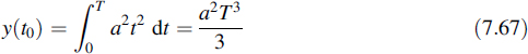
At the decision instant t0 the value of the output signal y(t0) equals the energy of the incoming signal till the moment t0, multiplied by an arbitrary constant that may be introduced in hopt(t).
The noise power at the output of the matched filter is
The last equality in this equation follows from Parseval's formula (see Appendix G or references [7] and [10]). However, since we found that the impulse response of the optimal filter is simply a mirrored version in time of the received signal (see Equation (7.56)) it is concluded that
with Ex the energy content of the signal x(t). From Equations (7.57) and (7.59) the signal-to-noise ratio at the output of the filter can be deduced.
Theorem 14
The signal-to-noise ratio at the output of the matched filter at the sampling instant is
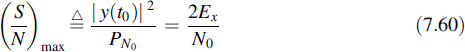
with Ex the energy content of the received signal and N0/2 the spectral density of the additive white noise.
Although a method exists to generalize the theory of Sections 7.1.2 and 7.1.3 to include coloured noise, we will present a simpler alternative here. This alternative reduces the problem of coloured noise to that of white noise, for which we now know the solution, as presented in the last paragraph. The basic idea is to insert a filter between the input and matched filter. The transfer function of this inserted filter is chosen such that the coloured input noise is transformed into white noise. The receiving filter scheme is as shown in Figure 7.6. It depicts the situation for hypothesis H1, with the input p(t) + N(t). The spectrum of N(t) is assumed to be coloured. Based on what we want to achieve, the transfer function of the first filter should satisfy

Figure 7.6 Matched filter for coloured noise
By means of Equation (4.27) it is readily seen that the noise N1(t) at the output of this filter has a white spectral density. For this reason the filter is called a whitening filter. The spectrum of the signal p1(t) at the output of this filter can be written as
The problem therefore reduces to the white noise case in Theorem 13. The filter H2(ω) has to be matched to the output of the filter H1(ω) and thus reads
In the second equation above we used the fact that SN1N1(ω) = 1, which follows from Equations (7.61) and (4.27). The matched filter for a known signal p(t) disturbed by coloured noise is found when using Equations (7.61) and (7.63):
It is concluded that the matched filter for a signal disturbed by coloured noise corresponds to the optimal filter from Equation (7.54).
Example 7.4:
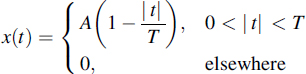
Consider the signal
This signal is shown in Figure 7.7(a). We want to characterize the matched filter for this signal when it is disturbed by white noise and to determine the maximum value of the signal-to-noise ratio. The sampling instant is chosen as t0 = 2T. In view of the simple description of the signal in the time domain it seems reasonable to do all the necessary calculations in the time domain. Illustrations of the different signals involved give a clear insight of the method. The signal x(−t) is in Figure 7.7(b) and from this follows the optimal filter characterized by its impulse response hopt(t), which is depicted in Figure 7.7(c). The maximum signal-to-noise ratio, occurring at the sampling instant t0, is calculated as follows. The noise power follows from Equation (7.58) yielding
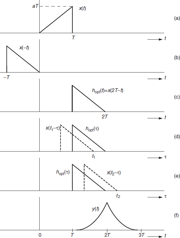
Figure 7.7 The different signals belonging to the example on a matched filter for the signal x(t) disturbed by white noise

The signal value at t = t0, using Equation (7.57), is
Using Equations (7.47), (7.66) and (7.67) the signal-to-noise ratio at the sampling instant t0 is

The output signal y(t) follows from the convolution of x(t) and hopt(t) as given by Equation (7.56). The convolution is
The various signals are shown in Figure 7.7. In Figure 7.7(d) the function hopt(τ) has been drawn, together with x(t − τ) for t = t1 ; the latter is shown as a dashed line. We distinguish two different situations, namely t < t0 = 2T and t > t0 = 2T. In Figure 7.7(e) the latter case has been depicted for t = t2. These pictures reveal that y(t) has an even symmetry with respect to t0 = 2T. That is why we confine ourselves to calculate y(t) for t ≤ 2T. Moreover, from the figures it is evident that y(t) equals zero for t < T and t > 3T. For T ≤ t ≤ 2T we obtain (see Figure 7.7(d))

The function Y(t) has been depicted in Figure 7.7(f). It is observed that the signal attains it maximum at t = 2T, the sampling instant.
![]()
The maximum of the output signal of a matched filter is always attained at t0 and y(t) always shows even symmetry with respect to t = t0.
7.3 THE CORRELATION RECEIVER
In the former section we derived the linear time-invariant filter that maximizes the signal-to-noise ratio; it was called a matched filter. It can be used as a receiver filter prior to detection. It was shown in Section 7.1.2 that sampling and comparing the filtered signal with the proper threshold provides optimum detection of data signals in Gaussian noise. Besides matched filtering there is yet another method used to optimize the signal-to-noise ratio and which serves as an alternative for the matched filter. The method is called correlation reception.
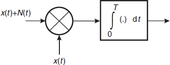
Figure 7.8 Scheme of the correlation receiver
The scheme of the correlation receiver is presented in Figure 7.8. In the receiver a synchronized replica of the information signal x(t) has to be produced; this means that the signal must be known by the receiver. The incoming signal plus noise is multiplied by the locally generated x(t) and the product is integrated. In the sequel we will show that the output of this system has the same signal-to-noise ratio as the matched filter.
For the derivation we assume that the pulse x(t) extends from t = 0 to t = T. Moreover, the noise process N(t) is supposed to be white with spectral density N0/2. Since the integration is a linear operation, it is allowed to consider the two terms of the product separately. Applying only x(t) to the input of the system of Figure 7.8 yields, at the output and at the sampling moment t0 = T, the quantity

where Ex is the energy in the pulse x(t).
Next we calculate the power of the output noise as

Then the signal-to-noise ratio is found from Equations (7.71) and (7.72) as

This is exactly the same as Equation (7.60).
From the point of view of S/N, the matched filter receiver and the correlation receiver behave identically. However, for practical application it is of importance to keep in mind that there are crucial differences. The correlation receiver needs a synchronized replica of the known signal. If such a replica cannot be produced or if it is not exactly synchronized, the calculated signal-to-noise ratio will not be achieved, yielding a lower value. Synchronization is the main problem in using the correlation receiver. In many carrier-modulated systems it is nevertheless employed, since in such situations the phased–locked loop provides an excellent expedient for synchronization. The big advantage of the correlation receiver is the fact that all the time it produces, apart from the noise, the squared value of the signal. Together with the integrator this gives a continuously increasing value of the output signal, which makes the receiver quite invulnerable to deviations from the optimum sampling instant. This is in contrast to the matched filter receiver. If, for instance, the information signal changes its sign, as is the case in modulated signals, then the matched filter output changes as well. In this case a deviation from the optimum sampling instant can result in the wrong decision about the information bit. This is clearly demonstrated by the next example.
Example 7.5:
In the foregoing it was shown that the matched filter and the correlation receiver have equal performance as far as the signal-to-noise ratios at the sampling instant is concerned. In this example we compare the outputs of the two receivers when an ASK modulated data signal has to be received. It suffices to consider a single data pulse isolated in time. Such a signal is written as
and where the symbol time T is an integer multiple of the period of the carrier frequency, i.e. T = n × 2π/ω0 and n is integer. As the sampling instant we take t0 = T. Then the matched filter output, for our purpose ignoring the noise, is found as

and
For other values of t the response is zero. The total response is given in Figure 7.9, with parameter values of A = T = 1, n = 4 and ω0 = 8π. Note the oscillating character of the response, which changes its sign frequently.

Figure 7.9 The response of the matched filter when driven by an ASK signal

Figure 7.10 Response of the correlation receiver to an ASK signal
Next we consider the response of the correlation receiver to the same ASK signal as input. Now we find
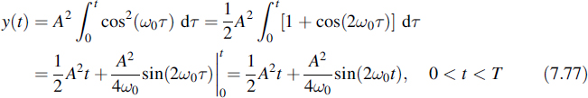
For negative values of t the response is zero and for t > T the response depends on the specific design of the receiver. In an integrate-and-dump receiver the signal is sampled and subsequently the value of the integrator output is reset to zero. The response of Equation (7.77) is presented in Figure 7.10 for the same parameters as used to produce Figure 7.9. Note that in this case the response is continuously non-decreasing, so no change of sign occurs. This makes this type of receiver much less vulnerable to timing jitter of the sampler. However, a perfect synchronization is required instead.
![]()
7.4 FILTERS THAT MINIMIZE THE MEAN-SQUARED ERROR
Thus far it was assumed that the signal to be detected had a known shape. Now we proceed with signals that are not known in advance, but the shape of the signal itself has to be estimated. Moreover, we assume as in the former case that the signal is corrupted by additive noise. Although the signal is not known in the deterministic sense, some assumptions will be made about its stochastic properties; the same holds for the noise. In this section we make an estimate of the received signal in the mean-squared sense, i.e. we minimize the mean-squared error between an estimate of the signal based on available data consisting of signal plus noise and the actual signal itself. As far as the signal processing is concerned we confine the treatment to linear filtering.
Two different problems are considered.
- In the first problem we assume that the data about the signal and noise are available for all times, so causality is ignored. We look for a linear time-invariant filtering that produces an optimum estimate for all times of the signal that is disturbed by the noise. This optimum linear filtering is called smoothing.
- In the second approach causality is taken into account. We make an optimum estimate of future values of the signal based on observations in the past up until the present time. Once more the estimate uses linear time-invariant filtering and we call the filtering prediction.
7.4.1 The Wiener Filter Problem
Based on the description in the foregoing we consider a realization S(t) of a wide-sense stationary process, called the signal. The signal is corrupted by the realization N(t) of another wide-sense stationary process, called the noise. Furthermore, the signal and noise are supposed to be jointly wide-sense stationary. The noise is supposed to be added to the signal. To the input of the estimator the process
is applied. When estimating the signal we base the estimate Ŝ(t + T) at some time t + T on a linear filtering of the input data X(t), i.e.

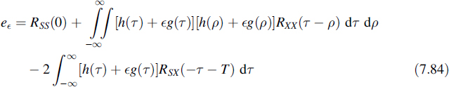
where h(τ) is the weighting function (equal to the impulse response of the linear time-invariant filter) and the integration limits a and b are to be determined later. Using Equation (7.79) the mean-squared error is defined as

Now the problem is to find the function h(τ) that minimizes the functional expression of Equation (7.80). In the minimization process the time shift T and integration interval are fixed; later on we will introduce certain restrictions to the shift and the integration interval, but for the time being they are arbitrary. The minimization problem can be solved by applying the calculus of variations [16]. According to this approach extreme values of the functional are achieved when the function h(τ) is replaced by h(τ) + ∈g(τ), where g(τ) is an arbitrary function of the same class as h(τ). Next the functional is differentiated with respect to ∈ and the result equated to zero for ∈ = 0. Solving the resulting equation produces the function h(τ), which leads to the extreme value of the functional. In the next subsections we will apply this procedure to the problem at hand.
7.4.2 Smoothing
In the smoothing (or filtering) problem it is assumed that the data (or observation) X(t) are known for the entire time axis −∞ < t < ∞. This means that there are no restrictions on the integration interval and we take a → −∞ and b → ∞. Expanding Equation (7.80) yields

Evaluating the expectations we obtain

and further

According to the calculus of variations we replace h(τ) by h(τ) + ∈g(τ) and obtain
The procedure proceeds by setting

After some straightforward calculations this leads to the solution
Since we assumed that the data are available over the entire time axis we can imagine that we apply this procedure on stored data. Moreover, in this case the integral in Equation (7.86) can be Fourier transformed as
Hence we do not need to deal with the integral equation, which is now transformed into an algebraic equation. For the filtering problem we can set T = 0 and the optimum filter follows immediately:
In the special case that the processes S(t) and N(t) are independent and at least one of these processes has zero mean, then the spectra can be written as

and as a consequence the optimum filter characteristic becomes
Once we have the expression for the optimum filter the mean-squared error of the estimate can be calculated. For this purpose multiply both sides of Equation (7.86) by hopt(τ) and integrate over τ. This reveals that, apart from the minus sign, the second term of Equation (7.83) is half of the value of the third term, so that
it is easy to see that
The Fourier transform of ξ(t) is
Hence the minimum mean-squared error is
When the special case of independence of the processes S(t) and N(t) is once more invoked, i.e. Equations (7.89) and (7.90) are inserted, then
Example 7.6:
A wide-sense stationary process has a flat spectrum within a limited frequency band, i.e.
The noise is independent of S(t) and has a white spectrum with a spectral density of N0/2. In this case the optimum smoothing filter has the transfer function

This result can intuitively be understood; namely the signal spectrum is completely passed undistorted by the ideal lowpass filter of bandwidth W and the noise is removed outside the signal bandwidth. The estimation error is

Interpreting S/N0 as the signal-to-noise ratio it is observed that the error decreases with increasing signal-to-noise ratios. For a large signal-to-noise ratio the error equals the noise power that is passed by the filter.
![]()
The filtering of an observed signal as described by Equation (7.91) is also called signal restoration. It is the most obvious method when the observation is available as stored data. When this is not the case, but an incoming signal has to be processed in real time, then the filtering given in Equation (7.88) can be applied, provided that the delay is so large that virtually the whole filter response extends over the interval −∞ < t < ∞. Despite the real-time processing, a delay between the arrival of the signal S(t) and the estimate of S(t − T) should be allowed. In that situation the optimum filter has an extra factor of exp(−jωT), which provides the delay, as follows from Equation (7.87). In general, a longer delay will reduce the estimation error, as long as the delay is shorter than the duration of the filter's impulse response h(τ).
7.4.3 Prediction
We now consider prediction based on the observation up to time t. Referring to Equation (7.79), we consider Ŝ(t + T) for positive values of T whereas X(t) is only known up to t. Therefore the integral limits in Equation (7.79) are a = −∞ and b = t. We introduce the causality of the filter's impulse response, given as
The general prediction problem is quite complicated [4]. Therefore we will confine the considerations here to the simplified case where the signal S(t) is not disturbed by noise, i.e. now we take N(t) ≡ 0. This is called pure prediction. It is easy to verify that in this case Equation (7.86) is reduced to
This equation is known as the Wiener–Hopf integral equation. The solution is not as simple as in former cases. This is due to the fact that Equation (7.102) is only valid for τ ≥ 0; therefore we cannot use the Fourier transform to solve it. The restriction τ ≥ 0 follows from Equation (7.84). In the case at hand the impulse response h(τ) of the filter is supposed to be causal and the auxiliary function g(τ) should be of the same class. Consequently, the solution now is only valid for τ ≥ 0. For τ < 0 the solution should be zero, and this should be guaranteed by the solution method.
Two approaches are possible for a solution. Firstly, a numerical solution can be invoked. For a fixed value of T the left-hand part of Equation (7.102) is sampled and the samples are collected in a vector. For the right-hand side RSS(τ − ρ) is sampled for each value of τ. The different vectors, one for each τ, are collected in a matrix, which is multiplied by the unknown vector made up from the sampled values of h(ρ). Finally, the solution is produced by matrix inversion.
Using an approximation we will also be able to solve it by means of the Laplace transform. Each function can arbitrarily be approximated by a rational function, the fraction of two polynomials. Let us suppose that the bilateral Laplace transform [7] of the auto-correlation function of S(t) is written as a rational function, i.e.
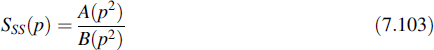
Since the spectrum is an even function it can be written as a function of p2. If we look at the positioning of zeros and poles in the complex p plane, it is revealed that this pattern is symmetrical with respect to the imaginary axis; i.e. if pi is a root of A(p2) then −pi is a root as well. The same holds for B(p2). Therefore SSS(p) can be factored as
where C(p) and D(p) comprise all the roots in the left half-plane and C(−p) and D(−p) the roots in the right half-plane, respectively; C(p) and C(−p) contain the roots of A2(p) and D(p) and D(−p) those of B2(p). For the sake of convenient treatment we suppose that all roots are simple. Moreover, we define
Both this function and its inverse are causal and realizable, since they are stable [7].
Let us now return to Equation (7.102), the integral equation to be solved. Rewrite it as
where f(τ) is a function that satisfies
i.e. f(τ) is anti-causal and analytic in the left-hand p plane (Re{p} < 0). The Laplace transform of Equation (7.106) is
where H(p) is the Laplace transform of h(t) and F(p) that of f(t). Solving this equation for H(p) yields
with the use of Equation (7.104). This function may only have roots in the left half-plane. If we select
then Equation (7.109) becomes
The choice given by Equation (7.110) guarantees that f(t) is anti-causal, i.e. f(t) = 0 for t ≥ 0. Moreover, making
satisfies one condition on H(p), namely that it is an analytic function in the right half-plane. Based on the numerator of Equation (7.111) we have to select N(p); for that purpose the data of D(p) can be used. We know that D(p) has all its roots in the left half-plane, so if we select N(p) such that its roots pi coincide with those of D(p) then the solution satisfies the condition that N(p) is an analytic function in the right half-plane. This is achieved when the roots pi are inserted in the numerator of Equation (7.111) to obtain
for all the roots pi of D(p). Connecting the roots of the solution in this way to the polynomial D(p) guarantees on the one hand that N(p) is analytic in the right half-plane and on the other hand satisfies Equation (7.111). This completes the selection of the optimum H(p).
Summarizing the method, we have to take the following steps:
- Factor the spectral function
where C(p) and D(p) comprise all the roots in the left half-plane and C(−p) and D(−p) the roots in the right half-plane, respectively.
- The denominator of the optimum filter H(p) has to be taken equal to C(p).
- Expand K(p) into partial fractions:
where pi are the roots of D(p).
- Construct the modified polynomial
- The optimum filter, described in the Laplace domain, then reads
Example 7.7:
Assume a process with the autocorrelation function
Then from a Laplace transform table it follows that
which is factored into

For the intermediate polynomial K(p) it is found that

Its constituting polynomials are
and
The polynomial C(p) has no roots and the only root of D(p) is p1 = −α. This produces

so that finally for the optimum filter we find
and the corresponding impulse response is
The minimum mean-squared error is given by substituting zero for the lower limit in the integral of Equation (7.92). This yields the error
![]()
This result reflects what may be expected, namely the facts that the error is zero when T = 0, which is actually no prediction, and that the error increases with increasing values of T.
7.4.4 Discrete-Time Wiener Filtering
Once the Wiener filter for continuous processes has been analysed, the time-discrete version follows straightforwardly. Equation (7.86) is the general solution for describing the different situations considered in this section. Its time-discrete version when setting the delay to zero is

Since this equation is valid for all n it is easily solved by taking the z-transform of both sides:
or

The error follows from the time-discrete counterparts of Equation (7.92) or Equation (7.96).
If both RXX[n] and RXS[n] have finite extent, let us say RXX[n] = RXS[n] = 0 for |n| > N, and if the extent of h[m] is limited to the same range, then Equation (7.128) can directly be solved in the time domain using matrix notation. For this case we define the (2N + 1) × (2N + 1) matrix as

Moreover, we define the (2N + 1) element vectors as
and
where ![]() and hT are the transposed vectors of the column vectors RXS and h, respectively.
and hT are the transposed vectors of the column vectors RXS and h, respectively.
By means of these definitions Equation (7.128) is rewritten as
with the solution for the discrete-time Wiener smoothing filter
This matrix description fits well in a modern numerical mathematical software package such as Matlab, which provides compact and efficient programming of matrices. Programs developed in Matlab can also be downloaded into DSPs, which is even more convenient.
Discrete-Time Prediction:
For the prediction problem a discrete-time version of the method presented in Subsection 7.4.3 can be developed (see reference [12]). However, using the time domain approach presented in the former paragraph, it is very easy to include noise; i.e. there is no need to limit the treatment to pure prediction.
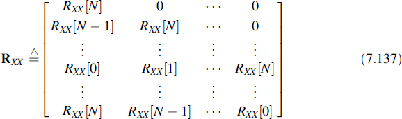
Once more we start from the discrete-time version of Equation (7.86), which is now written as

since the filter should be causal, i.e. h[m] = 0 for m < 0. Comparing this equation with Equation (7.128) reveals that they are quite similar. There is a time shift in RXS and a difference in the range of h[m]. For the rest the equations are the same. This means that the solution is also the same, provided that the matrix RXX and the vectors ![]() and hT are accordingly redefined. They become the (2N + 1) × (N + 1) matrix
and hT are accordingly redefined. They become the (2N + 1) × (N + 1) matrix
and the (2N + 1) element vector
respectively, and the (N + 1) element vector
The estimation error follows from the discrete-time version of Equation (7.92), which is

When the noise N[n] has zero mean and S[n] and N[n] are independent, they are orthogonal. This simplifies the cross-correlation of RSX to RSS.
7.5 SUMMARY
The optimal detection of binary signals disturbed by noise has been considered. The problem is reduced to hypothesis testing. When the noise has a Gaussian probability density function, we arrive at a special form of linear filtering, the so-called matched filtering. The optimum receiver for binary data signals disturbed by additive wide-sense stationary Gaussian noise consists of a matched filter followed by a sampler and a decision device.
Moreover, the matched filter can also be applied in situations where the noise (not necessarily Gaussian) has to be suppressed maximally compared to the signal value at a specific moment in time, called the sampling instant. Since the matched filter is in fact a linear time-invariant filter and the input noise is supposed to be wide-sense stationary, this means that the output noise variance is constant, i.e. independent of time, and that the signal attains its maximum value at the sampling instant. The name matched filter is connected to the fact that the filter characteristic (let it be described in the time or in the frequency domain) is determined by (matched to) both the shape of the received signal and the power spectral density of the disturbing noise.
Finally, filters that minimize the mean-squared estimation error (Wiener filters) have been derived. They can be used for smoothing of stored data or portions of a random signal that arrived in the past. In addition, filters that produce an optimal prediction of future signal values have been described. Such filters are derived both for continuous processes and discrete-time processes.
7.6 PROBLEMS
7.1 The input R = P + N is applied to a detector. The random variable P represents the information and is selected from P ∈ {+1, −0.5} and the selection occurs with the probabilities ![]() and
and ![]() The noise N has a triangular distribution fN(n) = tri(n).
The noise N has a triangular distribution fN(n) = tri(n).
(a) Make a sketch of the weighted (by the prior probabilities) conditional distribution functions.
(b) Determine the optimal decision regions.
(c) Calculate the minimum error probability.
7.2 Consider a signal detector with input R = P + N. The random variable P is the information and is selected from P ∈ {+A, −A}, with A a constant, and this selection occurs with equal probability. The noise N is characterized by the Laplacian probability density function

(a) Sketch the conditional probability density functions and determine the decision regions, without making a calculation.
(b) Consider the minimum probability of error receiver. Derive the probability of error for this receiver as a function of the parameters A and σ
(c) Determine the variance of the noise.
(d) Defining an appropriate signal-to-noise ratio S/N, determine the S/N to achieve an error probability of 10−5.
7.3 The M-ary PSK (phase shift keying) signal is defined as
![]()
where A and ω0 are constants representing the carrier amplitude and frequency, respectively, and i is randomly selected depending on the codeword to be transmitted. In Appendix A this signal is called a multiphase signal. This signal is disturbed by wide-sense stationary white Gaussian noise with spectral density N0/2.
(a) Make a picture of the signal constellation in the signal space for M = 8.
(b) Determine the decision regions and indicate them in the picture.
(c) Calculate the symbol error probability (i.e. the probability that a codeword is detected in error) for large values of the signal-to-noise ratio; assume, among others, that this error rate is dominated by transitions to nearest neighbours in the signal constellation. Express this error probability in terms of M, the mean energy in the codewords and the noise spectral density.
Hint: use Equation (5.65) for the probability density function of the phase.
7.4 A filter matched to the signal
has to be realized. The signal is disturbed by noise with the power spectral density
![]()
with A, T and W positive, real constants.
(a) Determine the Fourier transform of x(t).
(b) Determine the transfer function Hopt(ω) of the matched filter.
(c) Calculate the impulse response hopt(t). Sketch hopt(t).
(d) Is there any value of t0 for which the filter becomes causal? If so, what is that value?
7.5 The signal x(t) = u(t) exp(−Wt), with W > 0 and real, is applied to a filter together with white noise that has a spectral density of N0/2.
(a) Calculate the transfer function of the filter that is matched to x(t).
(b) Determine the impulse response of this filter. Make a sketch of it.
(c) Is there a value of t0 for which the filter becomes causal?
(d) Calculate the maximum signal-to-noise ratio at the output.
7.6 In a frequency domain description as given in Equation (7.54) the causality of the matched filter cannot be guaranteed. Using Equation (7.54) show that for a matched filter for a signal disturbed by (coloured) noise the following integral equation gives a time domain description:
![]()
where the causality of the filter can now be guaranteed by setting the lower bound of the integral equal to zero.
7.7 A pulse
![]()
is added to white noise N(t) with spectral density N0/2.
Find (S/N)max for a filter matched to x(t) and N(t).
7.8 The signal x(t) is defined as
![]()
This signal is disturbed by wide-sense stationary white noise with spectral density N0/2.
(a) Make a sketch of x(t).
(b) Sketch the impulse response of the matched filter if the sampling moment is t0 = T.
(c) Sketch the output signal y(t) of the filter.
(d) Calculate the signal-to-noise ratio at the filter output at t = t0.
(e) Show that the filter given in Problem 4.3 realizes the matched filter of this signal in white noise.
7.9 The signal x(t) is defined as
![]()
This signal is disturbed by wide-sense stationary white noise with spectral density N0/2.
(a) Make a sketch of x(t).
(b) Sketch the impulse response of the matched filter if the sampling moment is t0 = 3α.
(c) Calculate and sketch the output signal y(t) of the filter.
(d) Calculate the signal-to-noise ratio at the filter output at t = t0.
7.10 The signal x(t) is defined as

This signal is disturbed by wide-sense stationary white noise with spectral density N0/2.
(a) Make a sketch of x(t).
(b) Sketch the impulse response of the matched filter if the sampling moment is t0 = T.
(c) Sketch the output signal y(t) of the filter.
(d) Calculate the signal-to-noise ratio at the filter output at t = t0 and compare this with the outcome of Problem 7.8.
7.11 The signal p(t) is defined as
![]()
This signal is received twice (this is called ‘diversity’) in the following ways:
![]()
and
![]()
where α is a constant. The noise processes N1(t) and N2(t) are wide-sense stationary, white, independent processes and they both have the spectral density of N0/2. The signals R1(t) and R2(t) are received by means of matched filters. The outputs of the matched filters are sampled at t0 = T.
(a) Sketch the impulse responses of the two matched filters.
(b) Calculate the signal-to-noise ratios at the sample moments of the two individual receivers.
(c) By means of a new receiver design we produce the signal R3(t) = R1(t) + βR2(t), where β is a constant. Sketch the impulse response of the matched filter for R3(t) and calculate the signal-to-noise ratio at the sampling moment for this receiver.
(d) For what value of β will the signal-to-noise ratio from (c) attain its maximum value? (This is called ‘maximum ratio combining’.)
(e) Compare the signal-to-noise ratios from (b) with the maximum value found at (d) and explain eventual differences.
7.12 For the signal x(t) which is defined as
![]()
a matched filter has to be designed. As an approximation an RC filter is selected with the transfer function
![]()
with τ0 = RC. The disturbing noise is wide-sense stationary and white with spectral density N0/2.
(a) Calculate and sketch the output signal y(t) of the RC filter.
(b) Calculate the maximum value of the signal-to-noise ratio at the output of the filter. Find the value of τ0 that maximizes this signal-to-noise ratio.
Hint: use the Matlab command fsolve to solve the non-linear equation.
(c) Determine and sketch the output of the filter that is matched to the signal x(t).
(d) Calculate the signal-to-noise ratio of the matched filter output and determine the difference with that of the RC filter.
7.13 A binary transmission system, where ‘1’s and ‘0’s are transmitted, is disturbed by wide-sense stationary additive white Gaussian noise with spectral density N0/2. The ‘1’s are mapped on to the signal 3p(t) and ‘0’s on to p(t), where
![]()
In the binary received sequence those pulses will not overlap in time.
(a) Sketch p(t).
(b) Sketch the impulse response of the filter that is matched to p(t) and the noise, for the sampling moment t0 = T.
(c) Sketch y(t), the output of the filter when the input is p(t).
(d) Determine and sketch the conditional probability density functions when receiving a ‘0’ and a ‘1’, respectively.
(e) Calculate the bit error probability when the prior probabilities for sending a ‘1’ or a ‘0’ are equal and independent.
7.14 A binary transmission system, where ‘1’s and ‘0’s are transmitted, is disturbed by wide-sense stationary additive white Gaussian noise with spectral density N0/2. The ‘1’s are mapped on to the signal p(t) and the ‘0’s on to −p(t), where
![]()
In the binary received sequence those pulses will not overlap in time.
(a) Sketch p(t).
(b) Sketch the impulse response of the filter that is matched to p(t) and the noise, for the sampling moment t0 = T.
(c) Calculate and plot y(t), the output of the filter when the input is p(t).
(d) Determine and sketch the conditional probability density functions when receiving a ‘0’ or a ‘1’.
(e) Calculate the bit error probability when the prior probabilities for sending a ‘1’ or a ‘0’ are equal and independent.
7.15 Well-known digital modulation formats are ASK (amplitude shift keying) (see also Example 7.5) and PSK (phase shift keying). If we take one data symbol out of a sequence these formats are described by
![]()
where the bit levels A[n] are selected from A[n] ∈ {0, 1} for ASK and from A[n] ∈ {−1, 1} for PSK. The angular frequency ω0 is constant and T is the bit time. Moreover, it is assumed that T = n × 2π/ω0 with n an integer; i.e. the bit time is an integer number times the period of the carrier frequency. These signals are disturbed by wide-sense stationary white Gaussian noise with spectral density N0/2. Assume that the signals are detected by a correlation receiver, i.e. the received signal plus noise is multiplied by cos(ω0t) prior to detection.
(a) Sketch the signal constellations of ASK and PSK in signal space.
(b) Calculate the bit error rates, assuming the bits are equal probable. Express the error rates in terms of the mean energy in a bit and the spectral density of the noise.
7.16 An FSK (frequency shift keying) signal is defined as

where the bit levels A[n] are selected from A[n] ∈ {0, 1} and Ă[n] is the negated value of A[n], i.e. Ă[n] = 0 if A[n] = 1 and Ă[n] = 1 if A[n] = 0. The quantities ω1 and ω2 are constants and T is the bit time; the signal is disturbed by wide-sense stationary white Gaussian noise with spectral density N0/2. As in Problem 7.15, the signal is detected by a correlation receiver.
(a) Sketch the structure of the correlation receiver.
(b) What are the conditions for an orthogonal signals space?
(c) Sketch the signal constellation in the orthogonal signal space.
(d) Calculate the bit error rate expressed in the mean energy in a bit and the noise spectral density. Compare the outcome with that of ASK (Problem 7.15) and explain the similarity or difference.
7.17 The PSK system presented in Problem 7.15 is called BPSK (binary PSK) or phase reversal keying (PRK). Now consider an alternative scheme where the two possible phase realizations do not have opposite phases but are shifted π/2 in phase.
(a) Sketch the signal constellation in signal space and indicate the decision regions.
(b) Calculate the minimum bit error probability and compare it with that of BPSK. Explain the difference.
(c) Sketch the correlation receiver for this signal.
(d) Has this scheme advantages with respect to BPSK? What are the disadvantages?
7.18 A signal S(t) is observed in the middle of noise, i.e. X(t) = S(t) + N(t). The signal S(t) and the noise N(t) are jointly wide-sense stationary. Design an optimum smoothing filter to estimate the derivative S′(t) of the signal.
7.19 Derive the optimum prediction filter for a signal with spectral density
![]()
Introduction to Random Signals and Noise W. van
Etten © 2005 John Wiley & Sons, Ltd