
Contents
Overview of Generalized Linear Models
While traditional linear models are used extensively in statistical data analysis, there are types of problems for which they are not appropriate.
• It may not be reasonable to assume that data are normally distributed. For example, the normal distribution (which is continuous) may not be adequate for modeling counts or measured proportions.
• If the mean of the data is naturally restricted to a range of values, the traditional linear model may not be appropriate, since the linear predictor can take on any value. For example, the mean of a measured proportion is between 0 and 1, but the linear predictor of the mean in a traditional linear model is not restricted to this range.
• It may not be realistic to assume that the variance of the data is constant for all observations. For example, it is not unusual to observe data where the variance increases with the mean of the data.
A generalized linear model extends the traditional linear model and is, therefore, applicable to a wider range of data analysis problems. See the section Examples of Generalized Linear Models for the form of a probability distribution from the exponential family of distributions.
As in the case of traditional linear models, fitted generalized linear models can be summarized through statistics such as parameter estimates, their standard errors, and goodness-of-fit statistics. You can also make statistical inference about the parameters using confidence intervals and hypothesis tests. However, specific inference procedures are usually based on asymptotic considerations, since exact distribution theory is not available or is not practical for all generalized linear models.
The Generalized Linear Model Personality
Generalized linear models are fit as a personality of the Fit Model Dialog. After selecting Analyze > Fit Model, select Generalized Linear Model from the drop-down menu before or after assigning the effects to the model.
Figure 6.1 Generalized Linear Model Launch Dialog

When you specify that you are fitting a generalized linear model, the Fit Model dialog changes to allow you to select a Distribution and a Link Function. In addition, an Offset button, an option for overdispersion tests and intervals, and an option for Firth Bias-adjusted Estimates appears.
Examples of Generalized Linear Models
You construct a generalized linear model by deciding on response and explanatory variables for your data and choosing an appropriate link function and response probability distribution. Explanatory variables can be any combination of continuous variables, classification variables, and interactions.
|
Model
|
Response Variable
|
Distribution
|
Canonical Link Function
|
|
Traditional Linear Model
|
continuous
|
Normal
|
identity, g(μ) = μ
|
|
Logistic Regression
|
a count or a binary random variable
|
Binomial
|
logit,
|
|
Poisson Regression in Log Linear Model
|
a count
|
Poisson
|
log, g(μ) = log(μ)
|
|
Exponential Regression
|
positive continuous
|
Exponential
|
|
JMP fits a generalized linear model to the data by maximum likelihood estimation of the parameter vector. There is, in general, no closed form solution for the maximum likelihood estimates of the parameters. JMP estimates the parameters of the model numerically through an iterative fitting process. The dispersion parameter φ is also estimated by dividing the Pearson goodness-of-fit statistic by its degrees of freedom. Covariances, standard errors, and confidence limits are computed for the estimated parameters based on the asymptotic normality of maximum likelihood estimators.
A number of link functions and probability distributions are available in JMP. The built-in link functions are
identity: g(μ) = μ
logit:
probit: g(μ) = Φ-1(μ), where Φ is the standard normal cumulative distribution function
log: g(μ) = log(μ)
reciprocal: g(μ) =
power: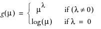
complementary log-log: g(m) = log(–log(1 – μ))
When you select the Power link function, a number box appears enabling you to enter the desired power.
The available distributions and associated variance functions are
normal: V(μ) = 1
binomial (proportion): V(μ) = μ(1 – μ)
Poisson: V(μ) = μ
Exponential: V(μ) = μ2
When you select Binomial as the distribution, the response variable must be specified in one of the following ways:
• If your data is not summarized as frequencies of events, specify a single binary column as the response. The response column must be nominal. If your data is summarized as frequencies of events, specify a single binary column as the response, along with a frequency variable in the Freq role. The response column must be nominal, and the frequency variable gives the count of each response level.
• If your data is summarized as frequencies of events and trials, specify two continuous columns in this order: a count of the number of successes, and a count of the number of trials. Alternatively, you can specify the number of failures instead of successes.
Model Selection and Deviance
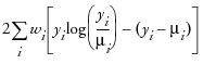
An important aspect of generalized linear modeling is the selection of explanatory variables in the model. Changes in goodness-of-fit statistics are often used to evaluate the contribution of subsets of explanatory variables to a particular model. The deviance, defined to be twice the difference between the maximum attainable log likelihood and the log likelihood at the maximum likelihood estimates of the regression parameters, is often used as a measure of goodness of fit. The maximum attainable log likelihood is achieved with a model that has a parameter for every observation. The following table displays the deviance for each of the probability distributions available in JMP.
|
Distribution
|
Deviance
|
|
normal
|
|
|
Poisson
|
 |
|
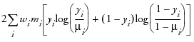
binomial1
|
 |
|
exponential
|
 |
1 In the binomial case, yi = ri /mi, where ri is a binomial count and mi is the binomial number of trials parameter
The Pearson chi-square statistic is defined as
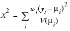
where yi is the ith response, μi is the corresponding predicted mean, V(μi) is the variance function, and wi is a known weight for the ith observation. If no weight is known, wi = 1 for all observations.
One strategy for variable selection is to fit a sequence of models, beginning with a simple model with only an intercept term, and then include one additional explanatory variable in each successive model. You can measure the importance of the additional explanatory variable by the difference in deviances or fitted log likelihoods between successive models. Asymptotic tests computed by JMP enable you to assess the statistical significance of the additional term.
Examples
The following examples illustrate how to use JMP’s generalized linear models platform.
Poisson Regression
This example uses data from a study of nesting horseshoe crabs. Each female crab had a male crab resident in her nest. This study investigated whether there were other males, called satellites, residing nearby. The data set CrabSatellites.jmp contains a response variable listing the number of satellites, as well as variables describing the female crab’s color, spine condition, weight, and carapace width. The data are shown in Figure 6.2.
Figure 6.2 Crab Satellite Data

To fit the Poisson loglinear model:
• Select Analyze > Fit Model
• Assign satell as Y
• Assign color, spine, width, and weight as Effects
• Choose the Generalized Linear Model Personality
• Choose the Poisson Distribution
The Log Link function should be selected for you automatically.
• Click Run.
The results are shown in Figure 6.3.
Figure 6.3 Crab Satellite Results
The Whole Model Test table gives information to compare the whole-model fit to the model that contains only the intercept parameter. The Reduced model is the model containing only an intercept. The Full model contains all of the effects as well as the intercept. The Difference is the difference of the log likelihoods of the full and reduced models. The Prob>Chisq is analogous to a whole-model F-test.
Second, goodness-of-fit statistics are presented. Analogous to lack-of-fit tests, they test for adequacy of the model. Low p-values for the ChiSquare goodness-of-fit statistics indicate that you may need to add higher-order terms to the model, add more covariates, change the distribution, or (in Poisson and binomial cases especially) consider adding an overdispersion parameter. AICc is also included and is the corrected Akaike’s Information Criterion, where
and k is the number of estimated parameters in the model and n is the number of observations in the data set. This value may be compared with other models to determine the best-fitting model for the data. The model having the smallest value, as discussed in Akaike (1974), is usually the preferred model.
The Effect Tests table shows joint tests that all the parameters for an individual effect are zero. If an effect has only one parameter, as with simple regressors, then the tests are no different from the tests in the Parameter Estimates table.
The Parameter Estimates table shows the estimates of the parameters in the model and a test for the hypothesis that each parameter is zero. Simple continuous regressors have only one parameter. Models with complex classification effects have a parameter for each anticipated degree of freedom. Confidence limits are also displayed.
Poisson Regression with Offset
The sample data table Ship Damage.JMP is adapted from one found in McCullugh and Nelder (1983). It contains information on a certain type of damage caused by waves to the forward section of the hull. Hull construction engineers are interested in the risk of damage associated with three variables: ship Type, the year the ship was constructed (Yr Made) and the block of years the ship saw service (Yr Used).
In this analysis we use the variable Service, the log of the aggregate months of service, as an offset variable. An offset variable is one that is treated like a regression covariate whose parameter is fixed to be 1.0.
These are most often used to scale the modeling of the mean in Poisson regression situations with log link. In this example, we use log(months of service) since one would expect that the number of repairs be proportional to the number of months in service. To see how this works, assume the linear component of the GLM is called eta. Then with a log link function, the model of the mean with the offset included is:
exp[Log(months of service) + eta] = [(months of service) * exp(eta)].
To run this example, assign
• Generalized Linear Model as the Personality
• Poisson as the Distribution, which automatically selects the Log link function
• N to Y
• Service to Offset
• Type, Yr Made, Yr Used as effects in the model
• Overdispersion Tests and Intervals with a check mark
The Fit Model dialog should appear like the one shown in Figure 6.4.
Figure 6.4 Ship Damage Fit Model Dialog

When you click Run, you see the report shown in Figure 6.5. Notice that all three effects (Type, Yr Made, Yr Used) are significant.
Figure 6.5 Ship Damage Report

Normal Regression, Log Link
Consider the following data set, where x is an explanatory variable and y is the response variable.
Figure 6.6 Nor.jmp data set

Using Fit Y By X, you can easily see that y varies nonlinearly with x and that the variance is approximately constant (see Figure 6.7). A normal distribution with a log link function is chosen to model these data; that is, log(μi) = xi'β so that μi = exp(xi'β). The completed Fit Model dialog is shown in Figure 6.8.
Figure 6.7 Y by X Results for Nor.jmp

Figure 6.8 Nor Fit Model Dialog

After clicking Run, you get the following report.
Figure 6.9 Nor Results
Because the distribution is normal, the Studentized Deviance residuals and the Deviance residuals are the same. To see this, select Diagnostic Plots > Deviance Residuals by Predicted from the platform drop-down menu.
Platform Commands
The following commands are available in the Generalized Linear Model report.
Custom Test allows you to test a custom hypothesis. Refer to Custom Test in the Fitting Standard Least Squares Models chapter for details on custom tests.
Contrast allows you to test for differences in levels within a variable. If a contrast involves a covariate, you can specify the value of the covariate at which to test the contrast.
In the Crab Satellite example, suppose you want to test whether the dark-colored crabs attracted a different number of satellites than the medium-colored crabs. Selecting Contrast brings up the following dialog.

Here you choose color, the variable of interest. When you click Go, you are presented with a Contrast Specification dialog.

To compare the dark-colored to the medium-colored, click the + button beside Dark and Dark Med, and the - button beside Medium and Light Medium.

Click Done to get the Contrast report shown here.

Since the Prob>Chisq is less than 0.05, we have evidence that there is a difference in satellite attraction based on color.
Inverse Prediction is used to predict an X value, given specific values for Y and the other X variables. This can be used to predict continuous variables only. For more details about Inverse Prediction, see Inverse Prediction in the Fitting Standard Least Squares Models chapter.
Covariance of Estimates produces a covariance matrix for all the effects in a model. The estimated covariance matrix of the parameter estimator is given by
Σ = -H-1
where H is the Hessian (or second derivative) matrix evaluated using the parameter estimates on the last iteration. Note that the dispersion parameter, whether estimated or specified, is incorporated into H. Rows and columns corresponding to aliased parameters are not included in Σ.
Correlation of Estimates produces a correlation matrix for all the effects in a model. The correlation matrix is the normalized covariance matrix. That is, if σij is an element of Σ, then the corresponding element of the correlation matrix is σij/σiσj, where
Profiler brings up the Profiler for examining prediction traces for each X variable. Details on the profiler are found in The Profiler in the Fitting Standard Least Squares Models chapter.
Contour Profiler brings up an interactive contour profiler. Details are found in Contour Profiler in the Visualizing, Optimizing, and Simulating Response Surfaces chapter.
Surface Profiler brings up a 3-D surface profiler. Details of Surface Plots are found in the Plotting Surfaces.
Diagnostic Plots is a submenu containing commands that allow you to plot combinations of residuals, predicted values, and actual values to search for outliers and determine the adequacy of your model. Deviance is discussed above in Model Selection and Deviance. The following plots are available:
• Studentized Deviance Residuals by Predicted
• Studentized Pearson Residuals by Predicted
• Deviance Residuals by Predicted
• Pearson Residuals By Predicted
• Actual by Predicted
• Regression Plot is available only when there is one continuous predictor and no more than one categorical predictor.
• Linear Predictor Plot is a plot of responses transformed by the inverse link function. This plot is available only when there is one continuous predictor and no more than one categorical predictor.
Save Columns is a submenu that lets you save certain quantities as new columns in the data table. Formuals for residuals are shown in Table 6.3.
|
Prediction Formula
|
Saves the formula that predicts the current model.
|
|
Predicted Values
|
Saves the values predicted by the current model.
|
|
Mean Confidence Interval
|
Saves the 95% confidence limits for the prediction equation. The confidence limits reflect variation in the parameter estimates.
|
|
Save Indiv Confid Limits
|
Saves the confidence limits for a given individual value. The confidence limits reflect variation in the error and variation in the parameter estimates.
|
|
Deviance Residuals
|
Saves the deviance residuals.
|
|
Pearson Residuals
|
Saves the Pearson residuals.
|
|
Studentized Deviance Residuals
|
Saves the studentized deviance residuals.
|
|
Studentized Pearson Residuals
|
Saves the studentized Pearson residuals.
|
|
(JSL only) Parametric Formula
|
Saves the parametric formula using JSL:
fit model object <<Parametric Formula( );
See the Object Scripting Index for an example.
|
|
Residual Type
|
Formula
|
|
Deviance
|
|
|
Studentized Deviance
|
 |
|
Pearson
|
 |
|
Studentized Pearson
|
 |
where (yi – μi) is the raw residual, sign(yi – μi) is 1 if (yi – μi) is positive and -1 if (yi – μi) is negative, di is the contribution to the total deviance from observation i, φ is the dispersion parameter, V(μi) is the variance function, and hi is the ith diagonal element of the matrix We(1/2)X(X'WeX)-1X'We(1/2), where We is the weight matrix used in computing the expected information matrix. For additional information regarding residuals and generalized linear models, see “The GENMOD Procedure” in the SAS/STAT User Guide documentation.
..................Content has been hidden....................
You can't read the all page of ebook, please click here login for view all page.