
Contents
Introduction to Partitioning
Variations of partitioning go by many names and brand names: decision trees, CARTTM, CHAIDTM, C4.5, C5, and others. The technique is often taught as a data mining technique because
• it is good for exploring relationships without having a good prior model,
• it handles large problems easily, and
• the results are very interpretable.
A classic application is where you want to turn a data table of symptoms and diagnoses of a certain illness into a hierarchy of questions to ask new patients in order to make a quick initial diagnosis.
The factor columns (X’s) can be either continuous or categorical (nominal or ordinal). If an X is continuous, then the splits (partitions) are created by a cutting value. The sample is divided into values below and above this cutting value. If the X is categorical, then the sample is divided into two groups of levels.
The response column (Y) can also be either continuous or categorical (nominal or ordinal). If Y is continuous, then the platform fits means. If Y is categorical, then the fitted value is a probability. In either case, the split is chosen to maximize the difference in the responses between the two branches of the split.
For more information on split criteria, see Statistical Details.
Launching the Partition Platform
To launch the Partition platform, select Analyze > Modeling > Partition. The Partition launch window is shown in Figure 13.2, using the Boston Housing.jmp data table.
Figure 13.2 Partition Launch Window
|
Option
|
Description
|
|
Y, Response
|
Choose the response variable.
|
|
X, Factor
|
Choose the predictor variables.
|
|
Validation
|
Enter a validation column here. For more information on validation, see Validation.
|
|
Missing Value Categories
|
Check this box to enable missing value categorization for nominal or ordinal predictors and responses. This option does not impact continuous predictors or responses.
For more details on this option, or for complete details on how the Partition platform handles missing values, see Missing Values.
|
|
Method
|
Select the partition method:
• Decision Tree
• Bootstrap Forest
• Boosted Tree
For more information on the methods, see Partition Method.
|
|
Validation Portion
|
Enter the portion of the data to be used as the validation set. For more information on validation, see Validation.
|
Partition Method
The Partition platform provides three methods for producing a final tree:
• For the Decision Tree method, see Decision Tree.
• For the Bootstrap Forest method, see Bootstrap Forest.
• For the Boosted Tree method, see Boosted Tree.
Decision Tree
The Decision Tree method makes a single pass through the data and produces a single tree. You can interactively grow the tree one split at a time, or grow the tree automatically if validation is used.
Decision Tree Report
As an example, use the Boston Housing.jmp data table. Launch the Partition platform and assign mvalue to the Y, Response role. Assign all the other variables to the X, Factor role. If using JMP Pro, select Decision Tree from the Method menu, then click OK. The initial report is shown in Figure 13.3.
Figure 13.3 Decision Tree Initial Report
The Split button is used to partition the data, creating a tree of partitions. Repeatedly splitting the data results in branches and leaves of the tree. This can be thought of as growing the tree. The Prune button is used to combine the most recent split back into one group.
Note the reported statistics:
RSquare
is the current R2 value.
N
is the number of observations (if no Freq variable is used).
Number of Splits
is the current number of splits.
AICc
is the corrected Akaike’s Information Criterion.
Count
gives the number of rows in the branch.
Mean
gives the average response for all rows in that branch.
Std Dev
gives the standard deviation of the response for all rows in that branch.
Initially, all rows are in one branch. In order to determine the first split, each X column must be considered. The candidate columns are shown in the Candidates report. As shown in Figure 13.4, the rooms column has the largest LogWorth, and is therefore the optimum split to make. See Statistical Details for more information about LogWorth.
Figure 13.4 Candidates Columns

The optimum split is noted by an asterisk. However, there are cases where the SS is higher for one variable, but the Logworth is higher for a different variable. In this case > and < are used to point in the best direction for each variable. The asterisk corresponds to the condition where they agree. See Statistical Details for more information about LogWorth and SS.
Click the Split button and notice the first split was made on the column rooms, at a value of 6.943. Open the two new candidate reports. See Figure 13.5.
Figure 13.5 First Split
The original 506 observations are now split into two parts:
• A left leaf, corresponding to rooms < 6.943, has 430 observations.
• A right leaf, corresponding to rooms ≥ 6.943, has 76 observations.
For the left leaf, the next split would happen on the column lstat, which has a SS of 7,311.85. For the right leaf, the next split would happen on the column rooms, which has a SS of 3,060.95. Since the SS for the left leaf is higher, using the Split button again will produce a split on the left leaf, on the column lstat.
Click the Split button to make the next split. See Figure 13.6.
Figure 13.6 Second Split
The 430 observations from the previous left leaf are now split into two parts:
• A left leaf, corresponding to lstat ≥ 14.43, has 175 observations.
• A right leaf, corresponding to lstat < 14.43, has 255 observations.
The 506 original observations are now split into three parts:
• A leaf corresponding to rooms < 6.943 and lstat ≥ 14.43.
• A leaf corresponding to rooms < 6.943 and lstat < 14.43.
• A leaf corresponding to rooms ≥ 6.943.
The predicted value for the observations in each leaf is the average response. The plot is divided into three sections, corresponding to the three leafs. These predicted values are shown on the plot with black lines. The points are put into random horizontal positions in each section. The vertical position is based on the response.
Stopping Rules
If validation is not used, the platform is purely interactive. Keep pushing the Split button until the result is satisfactory. Without cross-validation enabled, Partition is an exploratory platform intended to help you investigate relationships interactively.
When cross-validation is used, the user has the option to perform automatic splitting. This allows for repeated splitting without having to repeatedly click the Split button. See Automatic Splitting for details on the stopping rule.
Categorical Responses
When the response is categorical, the report differs in several ways (see Figure 13.7). The differences are described here, using the Car Poll.jmp data table:
• The G2 statistic is given instead of the Mean and Std Dev at the top of each leaf, and instead of SS in the Candidates report. See Statistical Details for more information about G2.
• The Rate statistic gives the proportion of observations in the leaf that are in each response level. The colored bars represent those proportions.
• The Prob statistic is the predicted value (a probability) for each response level. The Y axis of the plot is divided into sections corresponding to the predicted probabilities of the response levels for each leaf. The predicted probabilities always sum to one across the response levels. Random jitter is added to points in the X and Y direction in a leaf. See Statistical Details for more information about the Prob statistic.
• For the plot, the vertical position is random.
• The Color Points button appears. This colors the points on the plot according to the response levels.
Figure 13.7 Categorical Report
Node Options
This section describes the options on the red triangle menu of each node.
Split Best
finds and executes the best split at or below this node.
Split Here
splits at the selected node on the best column to split by.
Split Specific
lets you specify where a split takes place. This is useful in showing what the criterion is as a function of the cut point, as well as in determining custom cut points. After selecting this command, the following window appears.
Figure 13.8 Window for the Split Specific Command
The Split at menu has the following options:
Optimal Value splits at the optimal value of the selected variable.
Specified Value allows you to specify the level where the split takes place.
Output Split Table produces a data table showing all possible splits and their associated split value.
Prune Below
eliminates the splits below the selected node.
Prune Worst
finds and removes the worst split below the selected node.
Select Rows
selects the data table rows corresponding to this leaf. You can extend the selection by holding down the Shift key and choosing this command from another node.
Show Details
produces a data table that shows the split criterion for a selected variable. The data table, composed of split intervals and their associated criterion values, has an attached script that produces a graph for the criterion.
Lock
prevents a node or its subnodes from being chosen for a split. When checked, a lock icon is shown in the node title.
Platform Options
The section describes the options on the platform red triangle menu.
Display Options
gives a submenu consisting of items that toggle report elements on and off.
Show Points shows or hides the points. For categorical responses, this option shows the points or colored panels.
Show Tree shows or hides the large tree of partitions.
Show Graph shows or hides the partition graph.
Show Split Bar shows or hides the colored bars showing the split proportions in each leaf. This is for categorical responses only.
Show Split Stats shows or hides the split statistics. See Statistical Details for more information on the categorical split statistic G2.
Show Split Prob shows or hides the Rate and Prob statistics. This is for categorical responses only.
JMP automatically shows the Rate and Prob statistics when you select Show Split Count. See Statistical Details for more information on Rate and Prob.
Show Split Count shows or hides each frequency level for all nodes in the tree. This is for categorical responses only.
When you select this option, JMP automatically selects Show Split Prob. And when you deselect Show Split Prob, the counts do not appear.
Show Split Candidates shows or hides the Candidates report.
Sort Split Candidates sorts the candidates report by the statistic or the log(worth), whichever is appropriate. This option can be turned on and off. When off, it doesn’t change any reports, but new candidate reports are sorted in the order the X terms are specified, rather than by a statistic.
Split Best
splits the tree at the optimal split point. This is the same action as the Split button.
Prune Worst
removes the terminal split that has the least discrimination ability. This is equivalent to hitting the Prune Button.
Minimum Size Split
presents a dialog box where you enter a number or a fractional portion of the total sample size which becomes the minimum size split allowed. The default is 5. To specify a fraction of the sample size, enter a value less than 1. To specify an actual number, enter a value greater than or equal to 1.
Lock Columns
reveals a check box table to allow you to interactively lock columns so that they are not considered for splitting. You can toggle the display without affecting the individual locks.
Plot Actual by Predicted
produces a plot of actual values by predicted values. This is for continuous responses only.
Small Tree View
displays a smaller version of the partition tree to the right of the scatterplot.
Tree 3D
Shows or hides a 3D plot of the tree structure. To access this option, hold down the Shift key and click the red-triangle menu.
Leaf Report
gives the mean and count or rates for the bottom-level leaves of the report.
Column Contributions
brings up a report showing how each input column contributed to the fit, including how many times it was split and the total G2 or Sum of Squares attributed to that column.
Split History
shows a plot of R2 vs. the number of splits. If you use validation, separate curves are drawn for training and validation R2.
K Fold Crossvalidation
shows a Crossvalidation report, giving fit statistics for both the training and folded sets. For more information on validation, see Validation.
ROC Curve
is described in the section ROC Curve. This is for categorical responses only.
Lift Curve
is described in the section Lift Curves. This is for categorical responses only.
Show Fit Details
shows several measures of fit and a confusion matrix. The confusion matrix is a two-way classification of actual and predicted response. This is for categorical responses only.
Entropy RSquare compares the log-likelihoods from the fitted model and the constant probability model.
Generalized RSquare is a generalization of the Rsquare measure that simplifies to the regular Rsquare for continuous normal responses. It is similar to the Entropy RSquare, but instead of using the log-likelihood, it uses the 2/n root of the likelihood. It is scaled to have a maximum of 1. The value is 1 for a perfect model, and 0 for a model no better than a constant model.
Mean -Log p is the average of -log(p), where p is the fitted probability associated with the event that occurred.
RMSE is the root mean square error, where the differences are between the response and p (the fitted probability for the event that actually occurred).
Mean Abs Dev is the average of the absolute values of the differences between the response and p (the fitted probability for the event that actually occurred).
Misclassification Rate is the rate for which the response category with the highest fitted probability is not the observed category.
For Entropy RSquare and Generalized RSquare, values closer to 1 indicate a better fit. For Mean -Log p, RMSE, Mean Abs Dev, and Misclassification Rate, smaller values indicate a better fit.
Save Columns
is a submenu for saving model and tree results, and creating SAS code.
Save Residuals saves the residual values from the model to the data table.
Save Predicteds saves the predicted values from the model to the data table.
Save Leaf Numbers saves the leaf numbers of the tree to a column in the data table.
Save Leaf Labels saves leaf labels of the tree to the data table. The labels document each branch that the row would trace along the tree, with each branch separated by “&”. An example label could be “size(Small,Medium)&size(Small)”. However, JMP does not include redundant information in the form of category labels that are repeated. When a category label for a leaf references an inclusive list of categories in a higher tree node, JMP places a caret (‘^”) where the tree node with redundant labels occurs. Therefore, “size(Small,Medium)&size(Small)” is presented as ^&size(Small).
Save Prediction Formula saves the prediction formula to a column in the data table. The formula is made up of nested conditional clauses that describe the tree structure. The column includes a Response Probability property.
Save Tolerant Prediction Formula saves a formula that predicts even when there are missing values. The column includes a Response Probability property.
Save Leaf Number Formula saves a column containing a formula in the data table that computes the leaf number.
Save Leaf Label Formula saves a column containing a formula in the data table that computes the leaf label.
Make SAS DATA Step creates SAS code for scoring a new data set.
Make Tolerant SAS DATA Step creates SAS code that can score a data set with missing values.
Color Points
colors the points based on their response level. This is for categorical responses only, and does the same thing as the Color Points button (see Categorical Responses).
Script
contains options that are available to all platforms. See Using JMP.
Note: JMP 8 had a Partition Preference, and a Partition platform option, called Missing Value Rule. These have both been removed for JMP 9. The new method for handling missing values is described in Missing Values.
Automatic Splitting
The Go button (shown in Figure 13.9) appears when you have validation enabled. For more information on using validation, see Validation.
The Go button provides for repeated splitting without having to repeatedly click the Split button. When you click the Go button, the platform performs repeated splitting until the validation R-Square is better than what the next 10 splits would obtain. This rule may produce complex trees that are not very interpretable, but have good predictive power.
Using the Go button turns on the Split History command. If using the Go button results in a tree with more than 40 nodes, the Show Tree command is turned off.
Figure 13.9 The Go Button
Bootstrap Forest
The Bootstrap Forest method makes many trees, and averages the predicted values to get the final predicted value. Each tree is grown on a different random sample (with replacement) of observations, and each split on each tree considers only a random sample of candidate columns for splitting. The process can use validation to assess how many trees to grow, not to exceed the specified number of trees.
Another word for bootstrap-averaging is bagging. Those observations included in the growing of a tree are called the in-bag sample, abbreviated IB. Those not included are called the out-of-bag sample, abbreviated OOB.
Bootstrap Forest Fitting Options
If the Bootstrap Forest method is selected on the platform launch window, the Bootstrap Forest options window appears after clicking OK. Figure 13.10 shows the window using the Car Poll.jmp data table. The column sex is used as the response, and the other columns are used as the predictors.
Figure 13.10 Bootstrap Forest Fitting Options
The options on the Bootstrap Forest options window are described here:
Number of rows
gives the number of observations in the data table.
Number of terms
gives the number of columns specified as predictors.
Number of trees in the forest
is the number of trees to grow, and then average together.
Number of terms sampled per split
is the number of columns to consider as splitting candidates at each split. For each split, a new random sample of columns is taken as the candidate set.
Bootstrap sample rate
is the proportion of observations to sample (with replacement) for growing each tree. A new random sample is generated for each tree.
Minimum Splits Per Tree
is the minimum number of splits for each tree.
Minimum Size Split
is the minimum number of observations needed on a candidate split.
Early Stopping
is checked to perform early stopping. If checked, the process stops growing additional trees if adding more trees doesn’t improve the validation statistic. If not checked, the process continues until the specified number of trees is reached. This option appears only if validation is used.
Multiple Fits over number of terms
is checked to create a bootstrap forest for several values of Number of terms sampled per split. The lower value is specified above by the Number of terms samples per split option. The upper value is specified by the following option:
Max Number of terms is the maximum number of terms to consider for a split.
Bootstrap Forest Report
The Bootstrap Forest report is shown in Figure 13.11.
Figure 13.11 Bootstrap Forest
The results on the report are described here:
Model Validation - Set Summaries
provides fit statistics for all the models fit if you selected the Multiple Fits option on the options window.
Specifications
provides information on the partitioning process.
Overall Statistics
provides fit statistics for both the training and validation sets.
Confusion Matrix
provides two-way classifications of actual and predicted response levels for both the training and validation sets. This is available only with categorical responses.
Cumulative Validation
provides a plot of the fit statistics versus the number of trees. The Cumulative Details report below the plot is a tabulation of the data on the plot. This is only available when validation is used.
Per-Tree Summaries
gives summary statistics for each tree.
Bootstrap Forest Platform Options
The Bootstrap Forest report red-triangle menu has the following options:
Show Trees
is a submenu for displaying the Tree Views report. The report produces a picture of each component tree.
None does not display the Tree Views Report.
Show names displays the trees labeled with the splitting columns.
Show names categories displays the trees labeled with the splitting columns and splitting values.
Show names categories estimates displays the trees labeled with the splitting columns, splitting values, and summary statistics for each node.
Plot Actual by Predicted
provides a plot of actual versus predicted values. This is only for continuous responses.
Column Contributions
brings up a report showing how each input column contributed to the fit, including how many times it was split and the total G2 or Sum of Squares attributed to that column.
ROC Curve
is described in the section ROC Curve. This is for categorical responses only.
Lift Curve
is described in the section Lift Curves. This is for categorical responses only.
Save Columns
is a submenu for saving model and tree results, and creating SAS code.
Save Predicteds saves the predicted values from the model to the data table.
Save Prediction Formula saves the prediction formula to a column in the data table.
Save Tolerant Prediction Formula saves a formula that predicts even when there are missing values.
Save Residuals saves the residuals to the data table. This is for continuous responses only.
Save Cumulative Details creates a data table containing the fit statistics for each tree.
Make SAS DATA Step creates SAS code for scoring a new data set.
Make Tolerant SAS DATA Step creates SAS code that can score a data set with missing values.
Script
contains options that are available to all platforms. See Using JMP.
Boosted Tree
Boosting is the process of building a large, additive decision tree by fitting a sequence of smaller trees. Each of the smaller trees is fit on the scaled residuals of the previous tree. The trees are combined to form the larger final tree. The process can use validation to assess how many stages to fit, not to exceed the specified number of stages.
The tree at each stage is short, typically 1-5 splits. After the initial tree, each stage fits the residuals from the previous stage. The process continues until the specified number of stages is reached, or, if validation is used, until fitting an additional stage no longer improves the validation statistic. The final prediction is the sum of the estimates for each terminal node over all the stages.
If the response is categorical, the residuals fit at each stage are offsets of linear logits. The final prediction is a logistic transformation of the sum of the linear logits over all the stages.
For categorical responses, only those with two levels are supported.
Boosted Tree Fitting Options
If the Boosted Tree method is selected on the platform launch window, the Boosted Tree options window appears after clicking OK. See Figure 13.12.
Figure 13.12 Boosted Tree Options Window
The options on the Boosted Tree options window are described here:
Number of Layers
is the maximum number of stages to include in the final tree.
Splits per Tree
is the number of splits for each stage
Learning Rate
is a number such that 0 < r ≤ 1. Learning rates close to 1 result in faster convergence on a final tree, but also have a higher tendency to overfit data. Use learning rates closer to 1 when a small Number of Layers is specified.
Overfit Penalty
is a biasing parameter that helps to protect against fitting probabilities equal to zero.
Minimum Size Split
is the minimum number of observations needed on a candidate split.
Early Stopping
is checked to perform early stopping. If checked, the boosting process stops fitting additional stages if adding more stages doesn’t improve the validation statistic. If not checked, the boosting process continues until the specified number of stages is reached. This option is available only if validation is used.
Multiple Fits over splits and learning rate
is checked to create a boosted tree for every combination of Splits per Tree and Learning Rate. The lower ends of the combinations are specified by the Splits per Tree and Learning Rate options. The upper ends of the combinations are specified by the following options:
Max Splits Per Tree is the upper end for Splits per Tree.
Max Learning Rate is the upper end for Learning Rate.
Boosted Tree Report
The Boosted Tree report is shown in Figure 13.13.
Figure 13.13 Boosted Tree Report
The results on the report are described here:
Model Validation - Set Summaries
provides fit statistics for all the models fit if you selected the Multiple Splits option on the options window.
Specifications
provides information on the partitioning process.
Overall Statistics
provides fit statistics for both the training and validation sets.
Confusion Matrix
provides confusion statistics for both the training and validation sets. This is available only with categorical responses.
Cumulative Validation
provides a plot of the fit statistics versus the number of stages. The Cumulative Details report below the plot is a tabulation of the data on the plot. This is only available when validation is used.
Boosted Tree Platform Options
The Boosted Tree report red-triangle menu has the following options:
Show Trees
is a submenu for displaying the Tree Views report. The report produces a picture of the tree at each stage of the boosting process.
None does not display the Tree Views Report.
Show names displays the trees labeled with the splitting columns.
Show names categories displays the trees labeled with the splitting columns and splitting values.
Show names categories estimates displays the trees labeled with the splitting columns, splitting values, and summary statistics for each node.
Plot Actual by Predicted
provides a plot of actual versus predicted values. This is only for continuous responses.
Column Contributions
brings up a report showing how each input column contributed to the fit, including how many times it was split and the total G2 or Sum of Squares attributed to that column.
ROC Curve
is described in the section ROC Curve. This is for categorical responses only.
Lift Curve
is described in the section Lift Curves. This is for categorical responses only.
Save Columns
is a submenu for saving model and tree results, and creating SAS code.
Save Predicteds saves the predicted values from the model to the data table.
Save Prediction Formula saves the prediction formula to a column in the data table.
Save Tolerant Prediction Formula saves the prediction formula to a column in the data. This formula can predict even with missing values.
Save Residuals saves the residuals to the data table. This is for continuous responses only.
Save Offset Estimates saves the offsets from the linear logits. This is for categorical responses only.
Save Tree Details creates a data table containing split details and estimates for each stage.
Save Cumulative Details creates a data table containing the fit statistics for each stage.
Make SAS DATA Step creates SAS code for scoring a new data set.
Make Tolerant SAS DATA Step creates SAS code that can score a data set with missing values.
Script
contains options that are available to all platforms. See Using JMP.
Validation
If you grow a tree with enough splits, partitioning can overfit data. When this happens, the model predicts the fitted data very well, but predicts future observations poorly. Validation is the process of using part of a data set to estimate model parameters, and using the other part to assess the predictive ability of the model.
• The training set is the part that estimates model parameters.
• The validation set is the part that assesses or validates the predictive ability of the model.
• The test set is a final, independent assessment of the model’s predictive ability. The test set is available only when using a validation column (see Table 13.1).
The training, validation, and test sets are created by subsetting the original data into parts. Table 13.2 describes several methods for subsetting a data set.
|
Excluded Rows
|
Uses row states to subset the data. Rows that are unexcluded are used as the training set, and excluded rows are used as the validation set.
For more information about using row states and how to exclude rows, see Using JMP.
|
|
Holdback
|
Randomly divides the original data into the training and validation data sets. The Validation Portion (see Table 13.1) on the platform launch window is used to specify the proportion of the original data to use as the validation data set (holdback).
|
|
KFold
|
Divides the original data into K subsets. In turn, each of the K sets is used to validate the model fit on the rest of the data, fitting a total of K models. The model giving the best validation statistic is chosen as the final model.
KFold validation can be used only with the Decision Tree method. To use KFold, select K Fold Crossvalidation from the platform red-triangle menu, see Platform Options.
This method is best for small data sets, because is makes efficient use of limited amounts of data.
|
|
Validation Column
|
Uses a column’s values to divide the data into parts. The column is assigned using the Validation role on the Partition launch window. See Table 13.1.
The column’s values determine how the data is split, and what method is used for validation:
• If the column’s values are 0, 1and 2, then:
– Rows with 0 are assigned to the Training set
– Rows with 1 are assigned to the Validation set
– Rows with 2 are assigned to the Test set
• If the column’s values are 0 and 1, then only Training and Validation sets are used.
|
Graphs for Goodness of Fit
The graph for goodness of fit depends on which type of response you use. The Actual by Predicted plot is for continuous responses, and the ROC Curve and Lift Curve are for categorical responses.
Actual by Predicted Plot
For continuous responses, the Actual by Predicted plot shows how well the model fits the data. Each leaf is predicted with its mean, so the x-coordinates are these means. The actual values form a scatter of points around each leaf mean. A diagonal line represents the locus of where predicted and actual values are the same. For a perfect fit, all the points would be on this diagonal.
ROC Curve
The ROC curve is for categorical responses. The classical definition of ROC curve involves the count of True Positives by False Positives as you accumulate the frequencies across a rank ordering. The True Positive y-axis is labeled “Sensitivity” and the False Positive X-axis is labeled “1-Specificity”. The idea is that if you slide across the rank ordered predictor and classify everything to the left as positive and to the right as negative, this traces the trade-off across the predictor's values.
To generalize for polytomous cases (more than 2 response levels), Partition creates an ROC curve for each response level versus the other levels. If there are only two levels, one is the diagonal reflection of the other, representing the different curves based on which is regarded as the “positive” response level.
ROC curves are nothing more than a curve of the sorting efficiency of the model. The model rank-orders the fitted probabilities for a given Y-value, then starting at the lower left corner, draws the curve up when the row comes from that category, and to the right when the Y is another category.
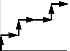
In the following picture, the Y axis shows the number of Y’s where Y=1, and the X axis shows the number of Y’s where Y=0.

If the model perfectly rank-orders the response values, then the sorted data has all the targeted values first, followed by all the other values. The curve moves all the way to the top before it moves at all to the right.
Figure 13.14 ROC for Perfect Fit

If the model does not predict well, it wanders more or less diagonally from the bottom left to top right.
In practice, the curve lifts off the diagonal. The area under the curve is the indicator of the goodness of fit, with 1 being a perfect fit.
If a partition contains a section that is all or almost all one response level, then the curve lifts almost vertically at the left for a while. This means that a sample is almost completely sensitive to detecting that level. If a partition contains none or almost none of a response level, the curve at the top will cross almost horizontally for a while. This means that there is a sample that is almost completely specific to not having that response level.
Because partitions contain clumps of rows with the same (i.e. tied) predicted rates, the curve actually goes slanted, rather than purely up or down.
For polytomous cases, you get to see which response categories lift off the diagonal the most. In the CarPoll example above, the European cars are being identified much less than the other two categories. The American's start out with the most sensitive response (Size(Large)) and the Japanese with the most negative specific (Size(Large)'s small share for Japanese).
Lift Curves
A lift curve shows the same information as an ROC curve, but in a way to dramatize the richness of the ordering at the beginning. The Y-axis shows the ratio of how rich that portion of the population is in the chosen response level compared to the rate of that response level as a whole. For example, if the top-rated 10% of fitted probabilities have a 25% richness of the chosen response compared with 5% richness over the whole population, the lift curve would go through the X-coordinate of 0.10 at a Y-coordinate of 25% / 5%, or 5. All lift curves reach (1,1) at the right, as the population as a whole has the general response rate.
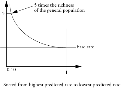
In problem situations where the response rate for a category is very low anyway (for example, a direct mail response rate), the lift curve explains things with more detail than the ROC curve.
Figure 13.15 Lift Curve
Missing Values
The Partition platform has methods for handling missing values in both Y and X variables.
Missing Responses
The handling of missing values for responses depends on if the response is categorical or continuous.
Categorical
If the Missing Value Categories checkbox (see Figure 13.2) is not selected, missing rows are not included in the analysis. If the Missing Value Categories checkbox is selected, the missing rows are entered into the analysis as another level of the variable.
Continuous
Rows with missing values are not included in the analysis.
Missing Predictors
The handling of missing values for predictors depends on if it is categorical or continuous.
Categorical
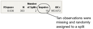
If the variable is used as a splitting variable, and if the Missing Value Categories checkbox (see Figure 13.2) is not selected, then each missing row gets randomly assigned to one of the two sides of the split. When this happens using the Decision Tree method, the Imputes message appears showing how many times this has happened. See Figure 13.16.
If the Missing Value Categories checkbox is selected, the missing rows are entered into the analysis as another level of the variable.
Continuous
If the variable is used as a splitting variable, then each missing row gets randomly assigned to one of the two sides of the split. When this happens using the Decision Tree method, the Imputes message appears showing how many times this has happened. See Figure 13.16.
Figure 13.16 Impute Message
Example
The examples in this section use the Boston Housing.jmp data table. Suppose you are interested in creating a model to predict the median home value as a function of several demographic characteristics.
The Partition platform can be used to quickly assess if there is any relationship between the response and the potential predictor variables. Build a tree using all three partitioning methods, and compare the results.
Note: Results will vary because the Validation Portion option chooses rows at random to use as the training and validation sets.
Decision Tree
Follow the steps below to grow a tree using the Decision Tree method:
1. Select Analyze > Modeling > Partition.
2. Assign mvalue to the Y, Response role.
3. Assign the other variables (crim through lstat) to the X, Factor role.
4.  Select the Decision Tree option from the Method menu. If using JMP, the Decision Tree option is the method that gets used.
5. Enter 0.2 for the Validation Portion.
6. Click OK.
7. On the platform report window, click Go to perform automatic splitting.
8. Select Plot Actual by Predicted from the platform red-triangle menu.
A portion of the report is shown in Figure 13.17.
Figure 13.17 Decision Tree Results
Bootstrap Forest
Follow the steps below to grow a tree using the Bootstrap Forest method:
1. Select Analyze > Modeling > Partition.
2. Assign mvalue to the Y, Response role.
3. Assign the other variables (crim through lstat) to the X, Factor role.
4. Select Bootstrap Forest from the Method menu.
5. Enter 0.2 for the Validation Portion.
6. Click OK.
7. Check the Early Stopping option on the Bootstrap Forest options window.
8. Click OK.
9. Select Plot Actual by Predicted from the red-triangle menu.
The report is shown in Figure 13.18.
Figure 13.18 Bootstrap Forest Report
Boosted Tree
Follow the steps below to grow a tree using the Boosted Tree method:
1. Select Analyze > Modeling > Partition.
2. Assign mvalue to the Y, Response role.
3. Assign the other variables (crim through lstat) to the X, Factor role.
4. Select Boosted Tree from the Method menu.
5. Enter 0.2 for the Validation Portion.
6. Click OK.
7. Check the Early Stopping option on the Boosted Tree options window.
8. Click OK.
9. Select Plot Actual by Predicted on the red-triangle menu.
The report is shown in Figure 13.19.
Figure 13.19 Boosted Tree Report
Compare Methods
The Decision Tree method produced a tree with 7 splits. The Bootstrap Forest method produced a final tree with 20 component trees. The Boosted Tree method produced a final tree with 50 component trees.
The Validation R-Square from the three methods are different, with the Boosted Tree having the best:
• Decision Tree 0.647
• Bootstrap Forest 0.716
• Boosted Tree 0.847
The actual-by-predicted plots show that the Boosted Tree method is best at predicting the actual median home values. The points on the plot are closer to the line for the Boosted Tree method.
Figure 13.20 shows a summary of the Column Contributions report from each method.
Figure 13.20 Column Contributions
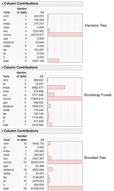
All three methods indicate that rooms and lstat are the most important variables for predicting median home value.
Statistical Details
This section provides some quantitative details and other information.
General
The response can be either continuous, or categorical (nominal or ordinal). If Y is categorical, then it is fitting the probabilities estimated for the response levels, minimizing the residual log-likelihood chi-square [2*entropy]. If the response is continuous, then the platform fits means, minimizing the sum of squared errors.
The factors can be either continuous, or categorical (nominal or ordinal). If an X is continuous, then the partition is done according to a splitting “cut” value for X. If X is categorical, then it divides the X categories into two groups of levels and considers all possible groupings into two levels.
Splitting Criterion
Node spliting is based on the LogWorth statistic, which is reported in node Candidate reports. LogWorth is calculated as:
-log10(p-value)
where the adjusted p-value is calculated in a complex manner that takes into account the number of different ways splits can occur. This calculation is very fair compared to the unadjusted p-value, which favors X’s with many levels, and the Bonferroni p-value, which favors X’s with small numbers of levels. Details on the method are discussed in a white paper “Monte Carlo Calibration of Distributions of Partition Statistics” found on the JMP website www.jmp.com.
For continuous responses, the Sum of Squares (SS) is reported in node reports. This is the change in the error sum-of-squares due to the split.
A candidate SS that has been chosen is
SStest = SSparent - (SSright + SSleft) where SS in a node is just s2(n - 1).
Also reported for continuous responses is the Difference statistic. This is the difference between the predicted values for the two child nodes of a parent node.
For categorical responses, the G2 (likelihood-ratio chi-square) is shown in the report. This is actually twice the [natural log] entropy or twice the change in the entropy. Entropy is Σ -log(p) for each observation, where p is the probability attributed to the response that occurred.
A candidate G2 that has been chosen is
G2 test = G2 parent - (G2 left + G2 right).
Partition actually has two rates; one used for training that is the usual ration of count to total, and another that is slightly biased away from zero. By never having attributed probabilities of zero, this allows logs of probabilities to be calculated on validation or excluded sets of data, used in Entropy RSquares.
Predicted Probabilities in Decision Tree and Bootstrap Forest
The predicted probabilities for the Decision Tree and Bootstrap Forest methods are calculated as described below by the Prob statistic.
For categorical responses in Decision Tree, the Show Split Prob command shows the following statistics:
Rate
is the proportion of observations at the node for each response level.
Prob
is the predicted probability for that node of the tree. The method for calculating Prob for the ith response level at a given node is as follows:
Probi =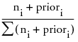
where the summation is across all response levels, ni is the number of observations at the node for the ith response level, and priori is the prior probability for the ith response level, calculated as
priori = λpi+ (1-λ)Pi
where pi is the priori from the parent node, Pi is the Probi from the parent node, and λ is a weighting factor currently set at 0.9.
The estimate, Prob, is the same that would be obtained for a Bayesian estimate of a multinomial probability parameter with a conjugate Dirichlet prior.
The method for calculating Prob assures that the predicted probabilities are always non-zero.
..................Content has been hidden....................
You can't read the all page of ebook, please click here login for view all page.