Contents
Overview of the Partial Least Squares Platform
The Partial Least Squares (PLS) platform fits linear models based on linear combinations, called factors, of the explanatory variables (Xs). These factors are obtained in a way that attempts to maximize the covariance between the Xs and the response or responses (Ys). In this way, PLS exploits the correlations between the Xs and the Ys to reveal underlying latent structures.
The PLS approach to model fitting is particularly useful when there are more explanatory variables than observations or when the explanatory variables are highly correlated. You can use PLS to fit a single model to several responses simultaneously. (Wold, 1995; Wold et al, 2001, Eriksson et al, 2006).
Two model fitting algorithms are available: nonlinear iterative partial least squares (NIPALS) and a “statistically inspired modification of PLS” (SIMPLS) (de Jong, 1993; Boulesteix and Strimmer, 2006). The SIMPLS algorithm was developed with the goal of solving a specific optimality problem. For a single response, both methods give the same model. For multiple responses, there are slight differences.
The platform uses the van der Voet T2 test and cross validation to help you choose the optimal number of factors to extract.
• In JMP, the platform uses the leave-one-out method of cross validation.
•  In JMP Pro, you can choose KFold or random holdback cross validation, or you can specify a validation column. If you prefer, you can also turn off validation. Note that leave-one-out cross validation can be obtained by setting the number of folds in KFold equal to the number of rows.
In JMP Pro, in addition to fitting main effects, you can also fit polynomial, interaction, and categorical effects by using the Partial Least Squares personality in Fit Model.
Example of Partial Least Squares
We consider an example from spectrometric calibration, and area where partial least squares is very effective. Consider the Baltic.jmp data table. The data are reported in Umetrics (1995); the original source is Lindberg, Persson, and Wold (1983). Suppose that you are researching pollution in the Baltic Sea. You would like to use the spectra of samples of sea water to determine the amounts of three compounds that are present in these samples. The three compounds of interest are: lignin sulfonate (ls), which is pulp industry pollution; humic acid (ha), a natural forest product; and an optical whitener from detergent (dt). The amounts of these compounds in each of the samples are the responses, The predictors are spectral emission intensities measured at a range of wavelengths (v1–v27).
For the purposes of calibrating the model, samples with known compositions are used. The calibration data consist of 16 samples of known concentrations of lignin sulfonate, humic acid, and detergent, with emission intensities recorded at 27 equidistant wavelengths. Use the Partial Least Squares platform to build a model for predicting the amount of the compounds from the spectral emission intensities.
In the following, we describe the steps and show reports for JMP. Because different cross validation options are used in JMP Pro, JMP Pro results for the default Model Launch settings differ from those shown in the figures below. To duplicate the results below in JMP Pro, in the Model Launch window, enter 16 as the Number of Folds under Validation Method and then click Go. This is equivalent to leave-one-out cross validation, which is the default method in JMP.
1. Open the Baltic.jmp sample data table.
2. Select Analyze > Multivariate Methods > Partial Least Squares.
3. Assign ls, ha, and dt to the Y, Response role.
4. Assign Intensities, which contains the 27 intensity variables v1 through v27, to the X, Factor role.
5. Click OK.
The Partial Least Squares Model Launch control panel appears.
6. Click Go.
A portion of the report appears in Figure 21.2.
Figure 21.2 Partial Least Squares Report

The JMP Standard platform uses leave-one-out cross validation in assessing the number of factors to extract. The Cross Validation report shows that the optimum number of factors to extract, based on Root Mean PRESS, is seven. A report entitled NIPALS Fit with 7 Factors is produced. A portion of that report is shown in Figure 21.3.
The van der Voet T2 statistic tests to determine whether a model with a different number of factors differs significantly from the model with the minimum PRESS value. Some authors recommend extracting the smallest number of factors for which the van der Voet significance level exceeds 0.10. Were you to apply this thinking in this example, you would fit a new model by entering 6 as the Number of Factors in the Model Launch window.
Figure 21.3 Seven Extracted Factors
7. Select Diagnostics Plots from the NIPALS Fit with 7 Factors red triangle menu.
This gives a report showing actual by predicted plots as well as three reports showing various residual plots. The Actual by Predicted Plot, shown in Figure 21.4, shows the degree to which predicted compound amounts agree with actual amounts.
Figure 21.4 Diagnostics Plots
Launch the Partial Least Squares Platform
There are two ways to launch the Partial Least Squares platform:
• Select Analyze > Multivariate Methods > Partial Least Squares. For details, see Launch through Multivariate Methods
•  Select Analyze > Fit Model and select Partial Least Squares from the Personality menu. For details, see Launching through Fit Model.
Launch through Multivariate Methods
To launch Partial Least Squares, select Analyze > Multivariate Methods > Partial Least Squares. Figure 21.5 shows the JMP Pro launch window for Baltic.jmp. The launch window in JMP does not provide the Validation or Impute Missing Data options.
Figure 21.5 Partial Least Squares Launch Window for JMP Pro
The launch window allows the following selections:
Y, Response
Enter the response columns.
X, Factor
Enter the X columns.
Validation
Allows the option to enter a validation column. If the validation column has more than two levels, then KFold Cross Validation is used. For information about other validation options, see Validation Method.
By
Allows the option to enter a column that creates separate reports for each level of the variable.
Centering
Subtracts the mean from each column. For more information, see Centering and Scaling.
Scaling
Divides each column by its standard deviation. For more information, see Centering and Scaling.
Impute Missing Data
Imputes values for observations with missing X values. For more information, see Impute Missing Data.
After completing the launch window and clicking OK, the Model Launch control panel appears. See Model Launch Control Panel.
Launching through Fit Model
In JMP Pro, you can launch Partial Least Squares through Fit Model. Select Analyze > Fit Model and select Partial Least Squares from the Personality menu. The options for Centering, Scaling, and Impute Missing Data appear in the Fit Model window, once the personality has been set to Partial Least Squares.
After completing the Fit Model window and clicking Run, the Model Launch control panel appears. See Model Launch Control Panel.
Note the following about using the Partial Least Squares personality of Fit Model:
• If you access Partial Least Squares through Fit Model, you can include categorical, polynomial, and interaction effects in the model.
• In JMP 10, the following Fit Model features are not available for the Partial Least Squares personality: Weight, Freq, Nest, Attributes, Transform, and No Intercept. The following Macros are not available: Response Surface, Mixture Response Surface, Scheffé Cubic, Radial.
Centering and Scaling
By default, the predictors and responses are centered and scaled to have mean 0 and standard deviation 1. Centering the predictors and the responses ensures that the criterion for choosing successive factors is based on how much variation they explain. Without centering, both the variable’s mean and its variation around that mean are involved in selecting factors.
Scaling places all predictors and responses on an equal footing relative to their variation. Suppose that Time and Temp are two of the predictors. Scaling them indicates that a change of one standard deviation in Time is approximately equivalent to a change of one standard deviation in Temp.
Impute Missing Data
Rows that are missing observations on any X variable are excluded from the analysis and no predictions are computed for these rows. Rows with no missing observations on X variables but with missing observations on Y variables are also excluded from the analysis, but predictions are computed.
However, JMP can compensate for missing observations on any X variable. Select Impute Missing Data on the PLS launch window. Missing data for the X variable is imputed using the average of the nonmissing values for that variable.
Model Launch Control Panel
After you click OK on the platform launch window (or Run in Fit Model), the Model Launch control panel appears (Figure 21.6). Note that the Validation Method portion of the Model Launch control panel has a different appearance in JMP Pro.
Figure 21.6 Partial Least Squares Model Launch Control Panel

The Model Launch control panel allows the following selections:
Method Specification
Select the type of model fitting algorithm. There are two algorithm choices: NIPALS and SIMPLS. The two methods produce the same coefficient estimates when there is only one response variable. See Statistical Details for differences between the two algorithms.
Validation Method
Select the validation method. Validation is used to determine the optimum number of factors to extract. For JMP Pro, if a validation column is specified on the platform launch window, these options do not appear.
Holdback Randomly selects the specified proportion of the data for fitting the model, and uses the other portion of the data to validate model fit.
KFold Partitions the data into K subsets, or folds. In turn, each fold is used to validate the model fit on the rest of the data, fitting a total of K models. This method is best for small data sets, because it makes efficient use of limited amounts of data.
Leave-One-Out Performs leave-one-out cross validation.
Note: In JMP Pro, leave-one-out cross validation can be obtained by setting the number of folds in KFold equal to the number of rows.
None Does not use validation to choose the number of factors to extract. The number of factors is specified in the Factor Search Range.
Factor Search Range
Specify how many latent factors to extract if not using validation. If validation is being used, this is the maximum number of factors the platform attempts to fit before choosing the optimum number of factors.
The Partial Least Squares Report
The first time you click Go in the Model Launch control panel (Figure 21.6), a new window appears that includes the control panel and three reports. You can fit additional models by specifying the desired numbers of factors in the control panel.
The following reports appear:
Model Comparison Summary
Displays summary results for each fitted model (Figure 21.7), where models for 7 and then 6 factors have been fit. The report includes the following summary information:
Method is the analysis method specified in the Model Launch control panel.
Number of rows is the number of observations used in the training set.
Number of factors is the number of extracted factors.
Percent Variation Explained for Cumulative X is the percent of variation in X explained by the model.
Percent Variation Explained for Cumulative Y is the percent of variation in Y explained by the model.
Number of VIP>0.8 is the number of X variables with VIP (variable importance for projection) values greater than 0.8. The VIP score is a measure of a variable’s importance relative to modeling both X and Y (Wold, 1995).
Figure 21.7 Model Comparison Summary

Cross Validation
This report only appears when cross validation is selected as a Validation Method in the Model Launch control panel. It shows summary statistics for models fit using from 0 to the maximum number of extracted factors, as specified in the Model Launch control panel (Figure 21.8). An optimum number of factors is identified using the minimum Root Mean PRESS (predicted residual sum of squares) statistic. The van der Voet T2 tests enable you to test whether models with different numbers of extracted factors differ significantly from the optimum model. The null hypothesis for each van der Voet T2 test states that the model based on the corresponding Number of factors does not differ from the optimum model. For more details, see van der Voet T2.
Figure 21.8 Cross Validation Report

Model Fit Report
Displays detailed results for each fitted model. The fit uses either the optimum number of factors based on cross validation, or the specified number of factors if no cross validation methods was specified. The report title indicates whether NIPALS or SIMPLS was used and gives the number of extracted factors.
The report includes the following summary information:
X-Y Scores Plots Produces scatterplots of the X and Y scores for each extracted factor.
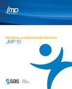
Percent Variation Explained Shows the percent variation and cumulative percent variation explained for both X and Y. Results are given for each extracted factor.
Model Coefficients for Centered and Scaled Data For each Y, shows the coefficients of the Xs for the model based on the centered and scaled data.
Model Coefficients for Original Data For each Y, shows the coefficients of the Xs for the model based on the original data.
Model Fit Options
The Model Fit red triangle menu has the following options:
Percent Variation Plots
Plots the percent variation explained by each extracted factor for the Xs and Ys.
Variable Importance Plot
Plots the VIP values for each X variable (Figure 21.9). The VIP score is a measure of a variable’s importance in modeling both X and Y. If a variable has a small coefficient and a small VIP, then it is a candidate for deletion from the model (Wold,1995). A value of 0.8 is generally considered to be a small VIP (Eriksson et al, 2006) and a blue line is drawn on the plot at 0.8.
Figure 21.9 Variable Importance Plot

VIP vs Coefficients Plots
Plots the VIP statistics against the model coefficients (Figure 21.10). Check boxes enable you to display only those points corresponding to your selected Ys. Additional labeling options are provided. There are plots for both the centered and scaled data and the original data.
To the right of the plot for the centered and scaled data are two options that facilitate variable reduction and model building. Make Model Using VIP opens and populates a launch window with the appropriate responses entered as Ys and the variables whose VIPs exceed the specified threshold entered as Xs. Make Model Using Selection enables you to select Xs directly in the plot and then enters the Ys and only the selected Xs into a launch window.
Figure 21.10 VIP vs Coefficients Plot for Centered and Scaled Data
Coefficient Plots
Plots the model coefficients for each response across the X variables (Figure 21.11). Check boxes allow you to display only those points corresponding to your selected Ys. There are plots for both the centered and scaled data and the original data.
Figure 21.11 Plot of Coefficients for Centered and Scaled Data
Loading Plots
Plots X and Y loadings for each extracted factor. There is a plot for the Xs and one for the Ys. The plot for the Xs is shown in Figure 21.12.
Figure 21.12 Plot of X Loadings

Loading Scatterplot Matrices
Shows a scatterplot matrix of the X loadings and a scatterplot matrix of the Y loadings.
Correlation Loading Plot
Shows a scatterplot matrix of the X and Y loadings overlaid on the same plot. Check boxes enable you to control labeling.
X-Y Score Plots
Includes the following options:
Fit Line Shows or hides a fitted line through the points on the X-Y Scores Plots.
Show Confidence Band Shows or hides 95% confidence bands for the fitted lines on the X-Y Scores Plots. Note that these should be used only for outlier detection.
Score Scatterplot Matrices
Shows a scatterplot matrix of the X scores and a scatterplot matrix of the Y scores. Each scatterplot displays a confidence ellipse. These may be used for outlier detection. For statistical details on the confidence ellipses, see Confidence Ellipse for Scatter Scores Plots.
Distance Plots
Shows a plot of the distance from each observation to the X model, the corresponding plot for the Y model, and a scatterplot of distances to both the X and Y models (Figure 21.13). In a good model, both X and Y distances are small, so the points are close to the origin (0,0). Use the plots to look for outliers relative to either X or Y. If a group of points clusters together, then they might have a common feature and could be analyzed separately.
Figure 21.13 Distance Plots

T Square Plot
Shows a plot of T2 statistics for each observation, along with a control limit. An observation’s T2 statistic is calculated based on that observation’s scores on the extracted factors. For details about the computation of T2 and the control limit, see T2 Plot.
Diagnostics Plots
Shows diagnostic plots for assessing the model fit. Four plot types are available: Actual by Predicted Plot, Residual by Predicted Plot, Residual by Row Plot, and a Residual Normal Quantile Plot (Figure 21.14). Plots are provided for each response
Figure 21.14 Diagnostics Plots

Profiler
shows a profiler for each Y variable.
Spectral Profiler
Shows a single profiler in which all the response variables are on the same plot. This is useful for visualizing the effect of changes in the X variables on the Y variables simultaneously.
Save Columns
Includes the following options for saving results:
Save Prediction Formula Saves the prediction formulas for the Y variables to columns in the data table.
Save Y Predicted Values Saves the predicted values for the Y variables to columns in the data table.
Save Y Residuals Saves the residual values for the Y variables to columns in the data table.
Save X Predicted Values Saves the predicted values for the X variables to columns in the data table.
Save X Residuals Saves the residual values for the X variables to columns in the data table.
Save Percent Variation Explained For X Effects Saves the percent variation explained for each X variable across all extracted factors to a new table.
Save Percent Variation Explained For Y Responses saves the percent variation explained for each Y variable across all extracted factors to a new table.
Save Scores Saves the X and Y scores for each extracted factor to the data table.
Save Loadings Saves the X and Y loadings to new data tables.
Save T Square Saves the T2 values to the data table. These are the values used in the T Square Plot.
Save Distance Saves the Distance to X Model (DModX) and Distance to Y Model (DModY) values to the data table. These are the values used in the Distance Plots.
Save X Weights Saves the weights for each X variable across all extracted factors to a new data table.
Save Validation Saves a new column to the data table describing how each observation was used in validation. For Holdback validation, the column identifies if a row was used for training or validation. For KFold validation, it identifies the number of the subgroup to which the row was assigned.
Remove Fit
Removes the model report from the main platform report.
Partial Least Squares Options
The Partial Least Squares red triangle menu has the following options:
Set Random Seed
In JMP Pro only. Sets the seed for the randomization process used for KFold and Holdback validation. This is useful if you want to reproduce an analysis. Set the seed to a positive value, save the script, and the seed is automatically saved in the script. Running the script will always produce the same cross validation analysis. This option does not appear when Validation Method is set to None, or when a validation column is used.
Script
Contains automation options that are available to all platforms. See the Using JMP book.
Statistical Details
This section provides details about some of the methods used in the Partial Least Squares platform.
Partial Least Squares
Partial least squares fits linear models based on linear combinations, called factors, of the explanatory variables (Xs). These factors are obtained in a way that attempts to maximize the covariance between the Xs and the response or responses (Ys). In this way, PLS exploits the correlations between the Xs and the Ys to reveal underlying latent structures. The factors address the combined goals of explaining response variation and predictor variation. Partial least squares is particularly useful when you have more X variables than observations or when the X variables are highly correlated.
NIPALS
The NIPALS method works by extracting one factor at a time. Let X = X0 be the centered and scaled matrix of predictors and Y = Y0 the centered and scaled matrix of response values. The PLS method starts with a linear combination t = X0w of the predictors, where t is called a score vector and w is its associated weight vector. The PLS method predicts both X0 and Y0 by regression on t:
The vectors p and c are called the X- and Y-loadings, respectively.
The specific linear combination t = X0w is the one that has maximum covariance t´u with some response linear combination u = Y0q. Another characterization is that the X- and Y-weights, w and q, are proportional to the first left and right singular vectors of the covariance matrix X0´Y0. Or, equivalently, the first eigenvectors of X0´Y0Y0´X0 and Y0´X0X0´Y0 respectively.
This accounts for how the first PLS factor is extracted. The second factor is extracted in the same way by replacing X0 and Y0 with the X- and Y-residuals from the first factor:
X1 = X0 –
Y1 = Y0 –
These residuals are also called the deflated X and Y blocks. The process of extracting a score vector and deflating the data matrices is repeated for as many extracted factors as are desired.
SIMPLS
The SIMPLS algorithm was developed to optimize a statistical criterion: it finds score vectors that maximize the covariance between linear combinations of Xs and Ys, subject to the requirement that the X-scores are orthogonal. Unlike NIPALS, where the matrices X0 and Y0 are deflated, SIMPLS deflates the cross-product matrix, X0´Y0.
In the case of a single Y variable, these two algorithms are equivalent. However, for multivariate Y, the models differ. SIMPLS was suggested by De Jong (1993).
T2 Plot
The T2 value for the ith observation is computed as follows:

where tij = X score for the ith row and jth extracted factor, p = number of extracted factors, and n = number of observations used to train the model. If validation is not used, n = total number of observations.
The control limit for the T2 Plot is computed as follows:
((n-1)2/n)*BetaQuantile(0.95, p/2, (n-p-1)/2)
where p = number of extracted factors, and n = number of observations used to train the model. If validation is not used, n = total number of observations.
van der Voet T2
The van der Voet T2 test helps determine whether a model with a specified number of extracted factors differs significantly from a proposed optimum model. The test is a randomization test based on the null hypothesis that the squared residuals for both models have the same distribution. Intuitively, one can think of the null hypothesis as stating that both models have the same predictive ability.
The test statistic is

where  is the jth predicted residual for response k for the model with i extracted factors, and
  is the corresponding quantity for the model based on the proposed optimum number of factors, opt. The significance level is obtained by comparing Ci with the distribution of values that results from randomly exchanging
  and
and  . A Monte Carlo sample of such values is simulated and the significance level is approximated as the proportion of simulated critical values that are greater than Ci.
Confidence Ellipse for Scatter Scores Plots
The Scatter Scores Plots option produces scatterplots with a confidence ellipse. The coordinates of the top, bottom, left, and right extremes of the ellipse are as follows:
For a scatterplot of score i versus score j:
• the top and bottom extremes are +/-sqrt(var(score i)*z)
• the left and right extremes are +/-sqrt(var(score j)*z)
where z = ((n-1)*(n-1)/n)*BetaQuantile(0.95, 1, (n-3)/2).
..................Content has been hidden....................
You can't read the all page of ebook, please click here login for view all page.