
Contents
Introduction to Logistic Models
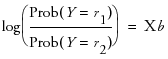
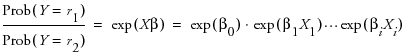
Logistic regression fits nominal Y responses to a linear model of X terms. To be more precise, it fits probabilities for the response levels using a logistic function. For two response levels, the function is:
or equivalently:
 where r1 and r2 are the two responses
For r nominal responses, where  , it fits
  sets of linear model parameters of the following form:
The fitting principal of maximum likelihood means that the βs are chosen to maximize the joint probability attributed by the model to the responses that did occur. This fitting principal is equivalent to minimizing the negative log-likelihood (–LogLikelihood) as attributed by the model:

For example, consider an experiment that was performed on metal ingots prepared with different heating and soaking times. The ingots were then tested for readiness to roll. See Cox (1970). The Ingots.jmp data table in the Sample Data folder has the experimental results. The categorical variable called ready has values 1 and 0 for readiness and not readiness to roll, respectively.
The Fit Model platform fits the probability of the not readiness (0) response to a logistic cumulative distribution function applied to the linear model with regressors heat and soak:
Probability (not ready to roll) =
The parameters are estimated by minimizing the sum of the negative logs of the probabilities attributed to the observations by the model (maximum likelihood).
To analyze this model, select Analyze > Fit Model. The ready variable is Y, the response, and heat and soak are the model effects. The count column is the Freq variable. When you click Run, iterative calculations take place. When the fitting process converges, the nominal or ordinal regression report appears. The following sections discuss the report layout and statistical tables, and show examples.
The Logistic Fit Report
Initially, the Logistic platform produces the following reports:
• Iterations
• Whole Model Test
• Lack of Fit (only if applicable)
• Parameter Estimates
• Effect Likelihood Ratio Tests
You can also request Wald Tests.
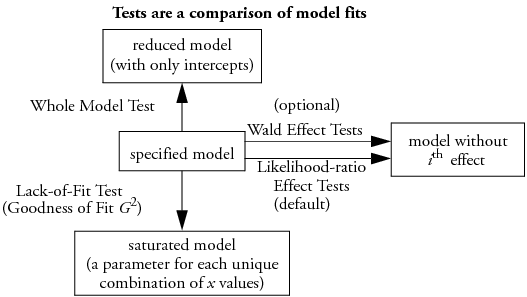
All tests compare the fit of the specified model with subset or superset models, as illustrated in Figure 7.1. If a test shows significance, then the higher order model is justified.
• Whole model tests: if the specified model is significantly better than a reduced model without any effects except the intercepts.
• Lack of Fit tests: if a saturated model is significantly better than the specified model.
• Effect tests: if the specified model is significantly better than a model without a given effect.
Figure 7.1 Relationship of Statistical Tables
Logistic Plot
If your model contains a single continuous effect, then a logistic report similar to the one in Fit Y By X appears. See Basic Analysis and Graphing for an interpretation of these plots.
Iteration History
After launching Fit Model, an iterative estimation process begins and is reported iteration by iteration. After the fitting process completes, you can open the Iteration report and see the iteration steps.
Figure 7.2 Iteration History
The Iterations history is available only for Nominal Logistic reports.
Whole Model Test
The Whole Model table shows tests that compare the whole-model fit to the model that omits all the regressor effects except the intercept parameters. The test is analogous to the Analysis of Variance table for continuous responses. The negative log-likelihood corresponds to the sums of squares, and the Chi-square test corresponds to the F test.
Figure 7.3 Whole Model Test

The Whole Model table shows these quantities:
Model
lists the model labels called Difference (difference between the Full model and the Reduced model), Full (model that includes the intercepts and all effects), and Reduced (the model that includes only the intercepts).
–LogLikelihood
records an associated negative log-likelihood for each of the models.
Difference is the difference between the Reduced and Full models. It measures the significance of the regressors as a whole to the fit.
Full describes the negative log-likelihood for the complete model.
Reduced describes the negative log-likelihood that results from a model with only intercept parameters. For the ingot experiment, the –LogLikelihood for the reduced model that includes only the intercepts is 53.49.
DF
records an associated degrees of freedom (DF) for the Difference between the Full and Reduced model. For the ingots experiment, there are two parameters that represent different heating and soaking times, so there are 2 degrees of freedom.
Chi-Square
is the Likelihood-ratio Chi-square test for the hypothesis that all regression parameters are zero. It is computed by taking twice the difference in negative log-likelihoods between the fitted model and the reduced model that has only intercepts.
Prob>ChiSq
is the probability of obtaining a greater Chi-square value by chance alone if the specified model fits no better than the model that includes only intercepts.
RSquare (U)
shows the R2, which is the ratio of the Difference to the Reduced negative log-likelihood values. It is sometimes referred to as U, the uncertainty coefficient. RSquare ranges from zero for no improvement to 1 for a perfect fit. A Nominal model rarely has a high Rsquare, and it has a Rsquare of 1 only when all the probabilities of the events that occur are 1.
AICc
is the corrected Akaike Information Criterion.
BIC
is the Bayesian Information Criterion
Observations
(or Sum Wgts) is the total number of observations in the sample.
Measure
gives several measures of fit to assess model accuracy.
Entropy RSquare is the same as R-Square (U) explained above.
Generalized RSquare is a generalization of the Rsquare measure that simplifies to the regular Rsquare for continuous normal responses. It is similar to the Entropy RSquare, but instead of using the log-likelihood, it uses the 2/n root of the likelihood.
Mean -Log p is the average of -log(p), where p is the fitted probability associated with the event that occurred.
RMSE is the root mean square error, where the differences are between the response and p (the fitted probability for the event that actually occurred).
Mean Abs Dev is the average of the absolute values of the differences between the response and p (the fitted probability for the event that actually occurred).
Misclassification Rate is the rate for which the response category with the highest fitted probability is not the observed category.
For Entropy RSquare and Generalized RSquare, values closer to 1 indicate a better fit. For Mean -Log p, RMSE, Mean Abs Dev, and Misclassification Rate, smaller values indicate a better fit.
After fitting the full model with two regressors in the ingots example, the –LogLikelihood on the Difference line shows a reduction to 5.82 from the Reduced –LogLikelihood of 53.49. The ratio of Difference to Reduced (the proportion of the uncertainty attributed to the fit) is 10.9% and is reported as the Rsquare (U).
To test that the regressors as a whole are significant (the Whole Model test), a Chi-square statistic is computed by taking twice the difference in negative log-likelihoods between the fitted model and the reduced model that has only intercepts. In the ingots example, this Chi-square value is  , and is significant at 0.003.
Lack of Fit Test (Goodness of Fit)
The next questions that JMP addresses are whether there is enough information using the variables in the current model or whether more complex terms need to be added. The Lack of Fit test, sometimes called a Goodness of Fit test, provides this information. It calculates a pure-error negative log-likelihood by constructing categories for every combination of the regressor values in the data (Saturated line in the Lack Of Fit table), and it tests whether this log-likelihood is significantly better than the Fitted model.
Figure 7.4 Lack of Fit Test
The Saturated degrees of freedom is m–1, where m is the number of unique populations. The Fitted degrees of freedom is the number of parameters not including the intercept. For the Ingots example, these are 18 and 2 DF, respectively. The Lack of Fit DF is the difference between the Saturated and Fitted models, in this case 18–2=16.
The Lack of Fit table lists the negative log-likelihood for error due to Lack of Fit, error in a Saturated model (pure error), and the total error in the Fitted model. Chi-square statistics test for lack of fit.
In this example, the lack of fit Chi-square is not significant (Prob>ChiSq = 0.617) and supports the conclusion that there is little to be gained by introducing additional variables, such as using polynomials or crossed terms.
Parameter Estimates
The Parameter Estimates report gives the parameter estimates, standard errors, and associated hypothesis test. The Covariance of Estimates report gives the variances and covariances of the parameter estimates.
Figure 7.5 Parameter Estimates Report

Likelihood Ratio Tests
The Likelihood Ratio Tests command produces a table like the one shown here. The Likelihood-ratio Chi-square tests are calculated as twice the difference of the log-likelihoods between the full model and the model constrained by the hypothesis to be tested (the model without the effect). These tests can take time to do because each test requires a separate set of iterations.
This is the default test if the fit took less than ten seconds to complete.
Figure 7.6 Effect Likelihood Ratio Tests

Logistic Fit Platform Options
The red triangle menu next to the analysis name gives you the additional options that are described next.
Plot Options
These options are described in the Basic Analysis and Graphing book.
Likelihood Ratio Tests
Wald Tests for Effects
One downside to likelihood ratio tests is that they involve refitting the whole model, which uses another series of iterations. Therefore, they could take a long time for big problems. The logistic fitting platform gives an optional test, which is more straightforward, serving the same function. The Wald Chi-square is a quadratic approximation to the likelihood-ratio test, and it is a by-product of the calculations. Though Wald tests are considered less trustworthy, they do provide an adequate significance indicator for screening effects. Each parameter estimate and effect is shown with a Wald test. This is the default test if the fit takes more than ten seconds to complete.
Figure 7.7 Effect Wald Tests

Likelihood-ratio tests are the platform default and are discussed under Likelihood Ratio Tests. It is highly recommended to use this default option.
Confidence Intervals
You can also request profile likelihood confidence intervals for the model parameters. When you select the Confidence Intervals command, a dialog prompts you to enter α to compute the 1 – α confidence intervals, or you can use the default of α = 0.05. Each confidence limit requires a set of iterations in the model fit and can be expensive. Furthermore, the effort does not always succeed in finding limits.
Figure 7.8 Parameter Estimates with Confidence Intervals

Odds Ratios (Nominal Responses Only)
When you select Odds Ratios, a report appears showing Unit Odds Ratios and Range Odds Ratios, as shown in Figure 7.9.
Figure 7.9 Odds Ratios

From the introduction (for two response levels), we had
 where r1 and r1 are the two response levels
so the odds ratio
Note that exp(βi(Xi + 1)) = exp(βiXi) exp(βi). This shows that if Xi changes by a unit amount, the odds is multiplied by exp(βi), which we label the unit odds ratio. As Xi changes over its whole range, the odds are multiplied by exp((Xhigh - Xlow)βi) which we label the range odds ratio. For binary responses, the log odds ratio for flipped response levels involves only changing the sign of the parameter, so you might want the reciprocal of the reported value to focus on the last response level instead of the first.
Two-level nominal effects are coded 1 and -1 for the first and second levels, so range odds ratios or their reciprocals would be of interest.
Dose Response Example
In the Dose Response.jmp sample data table, the dose varies between 1 and 12.
1. Open the Dose Response.jmp sample data table.
2. Select Analyze > Fit Model.
3. Select response and click Y.
4. Select dose and click Add.
5. Click OK.
6. From the red triangle next to Nominal Logistic Fit, select Odds Ratio.
Figure 7.10 Odds Ratios

The unit odds ratio for dose is 1.606 (which is exp(0.474)) and indicates that the odds of getting a Y = 0 rather than Y = 1 improves by a factor of 1.606 for each increase of one unit of dose. The range odds ratio for dose is 183.8 (exp((12-1)*0.474)) and indicates that the odds improve by a factor of 183.8 as dose is varied between 1 and 12.
Inverse Prediction
For a two-level response, the Inverse Prediction command finds the x value that results in a specified probability.
To see an example of inverse prediction:
1. Open the Ingots.jmp sample data table.
2. Select Analyze > Fit Y by X.
3. Select ready and click Y, Response.
4. Select heat and click X, Factor.
5. Select count and click Freq.
6. Click OK.
The cumulative logistic probability plot shows the result.
Figure 7.11 Logistic Probability Plot

Note that the fitted curve crosses the 0.9 probability level at a heat level of about 39.5, which is the inverse prediction. To be more precise and to get a fiducial confidence interval:
7. From the red triangle menu next to Logistic Fit, select Inverse Prediction.
8. For Probability, type 0.9.
9. Click OK.
The predicted value (inverse prediction) for heat is 39.8775, as shown in Figure 7.12.
Figure 7.12 Inverse Prediction Plot

However, if you have another regressor variable (Soak), you must use the Fit Model platform, as follows:
1. From the Ingots.jmp sample data table, select Analyze > Fit Model.
2. Select ready and click Y.
3. Select heat and soak and click Add.
4. Select count and click Freq.
5. Click Run.
6. From the red triangle next to Nominal Logistic Fit, select Inverse Prediction.
Then the Inverse Prediction command displays the Inverse Prediction window shown in Figure 7.13, for requesting the probability of obtaining a given value for one independent variable. To complete the dialog, click and type values in the editable X and Probability columns. Enter a value for a single X (heat or soak) and the probabilities that you want for the prediction. Set the remaining independent variable to missing by clicking in its X field and deleting. The missing regressor is the value that it will predict.
Figure 7.13 The Inverse Prediction Window and Table

See the appendix Statistical Details for more details about inverse prediction.
Save Commands
If you have ordinal or nominal response models, the Save Probability Formula command creates new data table columns.
If the response is numeric and has the ordinal modeling type, the Save Quantiles and Save Expected Values commands are also available.
The Save commands create the following new columns:
Save Probability Formula
creates columns in the current data table that save formulas for linear combinations of the response levels, prediction formulas for the response levels, and a prediction formula giving the most likely response.
For a nominal response model with r levels, JMP creates
• columns called Lin[j] that contain a linear combination of the regressors for response levels j = 1, 2, ... r - 1
• a column called Prob[r], with a formula for the fit to the last level, r
• columns called Prob[j] for j < r with a formula for the fit to level j
• a column called Most Likely responsename that picks the most likely level of each row based on the computed probabilities.
For an ordinal response model with r levels, JMP creates
• a column called Linear that contains the formula for a linear combination of the regressors without an intercept term
• columns called Cum[j], each with a formula for the cumulative probability that the response is less than or equal to level j, for levels j = 1, 2, ... r - 1. There is no Cum[ j = 1, 2, ... r - 1] that is 1 for all rows
• columns called Prob[ j = 1, 2, ... r - 1], for 1 < j < r, each with the formula for the probability that the response is level j. Prob[j] is the difference between Cum[j] and Cum[j –1]. Prob[1] is Cum[1], and Prob[r] is 1–Cum[r –1].
• a column called Most Likely responsename that picks the most likely level of each row based on the computed probabilities.
Save Quantiles
creates columns in the current data table named OrdQ.05, OrdQ.50, and OrdQ.95 that fit the quantiles for these three probabilities.
Save Expected Value
creates a column in the current data table called Ord Expected that is the linear combination of the response values with the fitted response probabilities for each row and gives the expected value.
ROC Curve
Receiver Operating Characteristic (ROC) curves measure the sorting efficiency of the model’s fitted probabilities to sort the response levels. ROC curves can also aid in setting criterion points in diagnostic tests. The higher the curve from the diagonal, the better the fit. An introduction to ROC curves is found in the Basic Analysis and Graphing book. If the logistic fit has more than two response levels, it produces a generalized ROC curve (identical to the one in the Partition platform). In such a plot, there is a curve for each response level, which is the ROC curve of that level versus all other levels. Details on these ROC curves are found in Graphs for Goodness of Fit in the Recursively Partitioning Data chapter.
Example of an ROC Curve
1. Open the Ingots.jmp sample data table.
2. Select Analyze > Fit Model.
3. Select ready and click Y.
4. Select heat and soak and click Add.
5. Select count and click Freq.
6. Click Run.
7. From the red triangle next to Nominal Logistic Fit, select ROC Curve.
8. Select 1 as the positive level and click OK.
Figure 7.14 ROC Curve

Lift Curve
Produces a lift curve for the model. A lift curve shows the same information as an ROC curve, but in a way to dramatize the richness of the ordering at the beginning. The Y-axis shows the ratio of how rich that portion of the population is in the chosen response level compared to the rate of that response level as a whole. See Lift Curves in the Recursively Partitioning Data chapter for more details about lift curves.
Figure 7.15 shows the lift curve for the same model specified for the ROC curve (Figure 7.14).
Figure 7.15 Lift Curve

Confusion Matrix
A confusion matrix is a two-way classification of the actual response levels and the predicted response levels. For a good model, predicted response levels should be the same as the actual response levels. The confusion matrix gives a way of assessing how the predicted responses align with the actual responses.
Profiler
Brings up the prediction profiler, showing the fitted values for a specified response probability as the values of the factors in the model are changed. This feature is available for both nominal and ordinal responses. For detailed information about profiling features, refer to the Visualizing, Optimizing, and Simulating Response Surfaces.
Validation
Validation is the process of using part of a data set to estimate model parameters, and using the other part to assess the predictive ability of the model.
• The training set is the part that estimates model parameters.
• The validation set is the part that assesses or validates the predictive ability of the model.
• The test set is a final, independent assessment of the model’s predictive ability. The test set is available only when using a validation column.
The training, validation, and test sets are created by subsetting the original data into parts. This is done through the use of a validation column in the Fit Model launch window.
The validation column’s values determine how the data is split, and what method is used for validation:
• If the column has two distinct values, then training and validation sets are created.
• If the column has three distinct values, then training, validation, and test sets are created.
• If the column has more than three distinct values, or only one, then no validation is performed.
When validation is used, model fit statistics are given for the training, validation, and test sets.
Example of a Nominal Logistic Model
A market research study was undertaken to evaluate preference for a brand of detergent (Ries and Smith 1963). The results are in the Detergent.jmp sample data table. The model is defined by the following:
• the response variable, brand with values m and x
• an effect called softness (water softness) with values soft, medium, and hard
• an effect called previous use with values yes and no
• an effect called temperature with values high and low
• a count variable, count, which gives the frequency counts for each combination of effect categories.
The study begins by specifying the full three-factor factorial model as shown by the Fit Model dialog in Figure 7.16. To specify a factorial model, highlight the three main effects in the column selector list. Then select Full Factorial from the Macros popup menu.
Figure 7.16 A Three-Factor Factorial Model with Nominal Response

Validation is available only in JMP Pro.
The tables in Figure 7.17 show the three-factor model as a whole to be significant (Prob>ChiSq = 0.0006) in the Whole Model table. The Effect Likelihood Ratio Tests table shows that the effects that include softness do not contribute significantly to the model fit.
Figure 7.17 Tables for Nominal Response Three-Factor Factorial

Next, use the Fit Model Dialog again to remove the softness factor and its interactions because they do not appear to be significant. You can do this easily by double-clicking the softness factor in the Fit Model dialog. A dialog appears, asking if you want to remove the other factors that involve softness (click Yes). This leaves the two-factor factorial model in Figure 7.18.
Figure 7.18 A Two-factor Factorial Model with Nominal Response

The Whole Model Test table shows that the two-factor model fits as well as the three-factor model. In fact, the three-factor Whole Model table in Figure 7.19 shows a larger Chi-square value (32.83) than the Chi-square value for the two-factor model (27.17). This results from the change in degrees of freedom used to compute the Chi-square values and their probabilities.
Figure 7.19 Two-Factor Model
The report shown in Figure 7.19 supports the conclusion that previous use of a detergent brand, and water temperature, have an effect on detergent preference, and the interaction between temperature and previous use is not statistically significant (the effect of temperature does not depend on previous use).
Example of an Ordinal Logistic Model
If the response variable has an ordinal modeling type, the platform fits the cumulative response probabilities to the logistic function of a linear model using maximum likelihood. Likelihood-ratio test statistics are provided for the whole model and lack of fit. Wald test statistics are provided for each effect.
If there is an ordinal response and a single continuous numeric effect, the ordinal logistic platform in Fit Y by X displays a cumulative logistic probability plot.
Details of modeling types are discussed in the Basic Analysis and Graphing book. The details of fitting appear in the appendix Statistical Details. The method is discussed in Walker and Duncan (1967), Nelson (1976), Harrell (1986), and McCullagh and Nelder (1983).
Note: If there are many response levels, the ordinal model is much faster to fit and uses less memory than the nominal model.
As an example of ordinal logistic model fitting, McCullagh and Nelder (1983) report an experiment by Newell to test whether various cheese additives (A to D) had an effect on taste. Taste was measured by a tasting panel and recorded on an ordinal scale from 1 (strong dislike) to 9 (excellent taste). The data are in the Cheese.jmp sample data table.
1. Open the Cheese.jmp sample data table.
2. Select Analyze > Fit Model.
3. Select Response and click Y.
4. Select Cheese and click Add.
5. Select Count and click Freq.
6. Click Run.
7. From the red triangle next to Ordinal Logistic Fit, select Wald Tests.
Figure 7.20 Ordinal Logistic Fit
The model in this example reduces the –LogLikelihood of 429.9 to 355.67. This reduction yields a likelihood-ratio Chi-square for the whole model of 148.45 with 3 degrees of freedom, showing the difference in perceived cheese taste to be highly significant.
The Lack of Fit test happens to be testing the ordinal response model compared to the nominal model. This is because the model is saturated if the response is treated as nominal rather than ordinal, giving 21 additional parameters, which is the Lack of Fit degrees of freedom. The nonsignificance of Lack of Fit leads one to believe that the ordinal model is reasonable.
There are eight intercept parameters because there are nine response categories. There are only three structural parameters. As a nominal problem, there are  structural parameters.
When there is only one effect, its test is equivalent to the Likelihood-ratio test for the whole model. The Likelihood-ratio Chi-square is 148.45, different from the Wald Chi-square of 115.15, which illustrates the point that Wald tests are to be regarded with some skepticism.
To see whether a cheese additive is preferred, look for the most negative values of the parameters (Cheese D’s effect is the negative sum of the others, shown in Figure 7.1.).
|
Cheese
|
Estimate
|
Preference
|
|
A
|
–0.8622
|
2nd place
|
|
B
|
2.4896
|
least liked
|
|
C
|
0.8477
|
3rd place
|
|
D
|
–2.4750
|
most liked
|
You can also use the Fit Y by X platform for this model, which treats ordinal responses like nominal and shows a contingency table analysis. See Figure 7.21. The Fit Model platform can also be used, but you must change the ordinal response, Response, to nominal. See Figure 7.22. Nominal Fit Model results are shown in Figure 7.22. Note that the negative log-likelihood values (84.381) and the likelihood chi-square values (168.76) are the same.
Figure 7.21 Fit Y by X Platform Results for Cheese.jmp
Figure 7.22 Fit Model Platform Results Setting Response to Nominal for Cheese.jmp
If you want to see a graph of the response probabilities as a function of the parameter estimates for the four cheeses, add the Score variable as a response surface effect to the Fit Model dialog as shown. To create the model in Figure 7.23, select Score in the column selector list, and then select Response Surface from the Macros popup menu on the Fit Model dialog.
Figure 7.23 Model Dialog For Ordinal Logistic Regression
Validation is available only in JMP Pro.
Click Run to see the analysis report and the cumulative logistic probability plot in Figure 7.24. The distance between each curve is the fitted response probability for the levels in the order for the levels on the right axis of the plot.
Figure 7.24 Cumulative Probability Plot for Ordinal Logistic Regression

Example of a Quadratic Ordinal Logistic Model
The Ordinal Response Model can fit a quadratic surface to optimize the probabilities of the higher or lower responses. The arithmetic in terms of the structural parameters is the same as that for continuous responses. Up to five factors can be used, but this example has only one factor, for which there is a probability plot.
Consider the case of a microwave popcorn manufacturer who wants to find out how much salt consumers like in their popcorn. To do this, the manufacturer looks for the maximum probability of a favorable response as a function of how much salt is added to the popcorn package. An experiment controls salt amount at 0, 1, 2, and 3 teaspoons, and the respondents rate the taste on a scale of 1=low to 5=high. The optimum amount of salt is the amount that maximizes the probability of more favorable responses. The ten observations for each of the salt levels are shown in Table 7.2.
|
Salt Amount
|
Salt Rating Response
|
|||||||||
|
no salt
|
1
|
3
|
2
|
4
|
2
|
2
|
1
|
4
|
3
|
4
|
|
1 tsp.
|
4
|
5
|
3
|
4
|
5
|
4
|
5
|
5
|
4
|
5
|
|
2 tsp.
|
4
|
3
|
5
|
1
|
4
|
2
|
5
|
4
|
3
|
2
|
|
3 tsp.
|
3
|
1
|
2
|
3
|
1
|
2
|
1
|
2
|
1
|
2
|
Use Fit Model with the Salt in Popcorn.jmp sample data to fit the ordinal taste test to the surface effect of salt. Use Taste Test as Y. Highlight Salt in the Select Columns box, and then select Macros > Response Surface.
The report shows how the quadratic model fits the response probabilities. The curves, instead of being shifted logistic curves, become a folded pile of curves where each curve achieves its optimum at the same point. The critical value is at Mean(X)–0.5 *b1/b2 where b1 is the linear coefficient and b2 is the quadratic coefficient. This formula is for centered X. From the Parameter Estimates table, you can compute the optimum as 1.5 - 0.5* (0.5637/1.3499) = 1.29 teaspoons of salt.
Figure 7.25 Ordinal Logistic Fit for Salt in Popcorn.jmp

The distance between each curve measures the probability of each of the five response levels. The probability for the highest response level is the distance from the top curve to the top of the plot rectangle. This distance reaches a maximum when the amount of salt is about 1.3 teaspoons. All curves share the same critical point.
The parameter estimates for Salt and Salt*Salt become the coefficients used to find the critical value. Although it appears as a minimum, it is only a minimum with respect to the probability curves. It is really a maximum in the sense of maximizing the probability of the highest response. The Solution portion of the report is shown under Response Surface in Figure 7.25, where 1.29 is shown under Critical Value.
Stacking Counts in Multiple Columns
Data that are frequencies (counts) listed in several columns of your data table are not the form that you need for logistic regression. For example, the Ingots2.jmp data table in the data folder (see Figure 7.26) has columns Nready and Nnotready that give the number of ready and number of not ready ingots for each combination of Heat and Soak values. To do a logistic regression, you need the data organized like the table in Figure 7.27.
To make a new table, suitable for logistic regression, select the Stack command from the Tables menu. Complete the Stack dialog by choosing Nready and NNotReady as the columns to stack, and then click OK in the Stack dialog. This creates the new table in Figure 7.27. If you use the default column names, Label is the response (Y) column and Data is the frequency column.
The example in the section Introduction to Logistic Models, shows a logistic regression using a sample data table Ingots.jmp. It has a frequency column called count (equivalent to the Data column in the table below) and a response variable called Ready, with values 1 to represent ingots that are ready and 0 for not ready.
Figure 7.26 Original Data Table

Figure 7.27 Stacked Data Table

..................Content has been hidden....................
You can't read the all page of ebook, please click here login for view all page.