Contents
Overview of the Loglinear Variance Model
The loglinear-variance model (Harvey 1976, Cook and Weisberg 1983, Aitken 1987, Carroll and Ruppert 1988) provides a way to model the variance simply through a linear model. In addition to having regressor terms to model the mean response, there are regressor terms in a linear model to model the log of the variance:
mean model: E(y) = Xβ
variance model: log(Variance(y)) = Z λ,
or equivalently
Variance(y) = exp(Z λ)
where the columns of X are the regressors for the mean of the response, and the columns of Z are the regressors for the variance of the response. The regular linear model parameters are represented by β, and λ represents the parameters of the variance model.
Log-linear variance models are estimated using REML.
A dispersion or log-variance effect can model changes in the variance of the response. This is implemented in the Fit Model platform by a fitting personality called the Loglinear Variance personality.
Model Specification
Log-linear variance effects are specified in the Fit Model dialog by highlighting them and selecting LogVariance Effect from the Attributes drop-down menu. &LogVariance appears at the end of the effect. When you use this attribute, it also changes the fitting Personality at the top to LogLinear Variance. If you want an effect to be used for both the mean and variance of the response, then you must specify it twice, once with the LogVariance option.
The effects you specify with the log-variance attribute become the effects that generate the Z’s in the model, and the other effects become the X’s in the model.
Notes
Every time another parameter is estimated for the mean model, at least one more observation is needed, and preferably more. But with variance parameters, several more observations for each variance parameter are needed to obtain reasonable estimates. It takes more data to estimate variances than it does means.
The log-linear variance model is a very flexible way to fit dispersion effects, and the method deserves much more attention than it has received so far in the literature.
Example Using Loglinear Variance
The data table InjectionMolding.jmp contains the experimental results from a 7-factor 27-3 fractional factorial design with four added centerpoints [from Myers and Montgomery, 1995, page 519, originally Montgomery, 1991]. Preliminary investigation determined that the mean response only seemed to vary with the first two factors, Mold Temperature, and Screw Speed, and the variance seemed to be affected by Holding Time.
Figure 12.1 Injection Molding Data

1. Open the InjectionMolding.jmp sample data table.
2. Select Analyze > Fit Model.
Since the variables in the data table have preselected roles assigned to them, the launch window is already filled out.
Figure 12.2 Fit Model Dialog

3. Click Run.
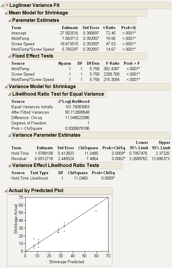
Figure 12.3 Loglinear Variance Report Window

The Mean Model for Shrinkage report gives the parameters for the mean model, and the Variance Model for Shrinkage report gives the parameters for the variance model.
The Loglinear Report
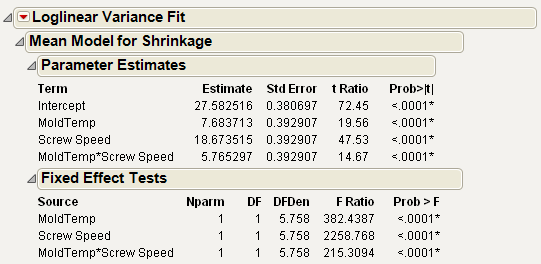
The top portion of the resulting report shows the fitting of the Expected response, with reports similar to standard least squares, though actually derived from restricted maximum likelihood (REML).
Figure 12.4 Mean Model Output

Figure 12.5 Variance Model Output

The second portion of the report shows the fit of the variance model. The Variance Parameter Estimates report shows the estimates and relevant statistics. Two hidden columns are provided:
• The hidden column exp(Estimate) is the exponential of the estimate. So, if the factors are coded to have +1 and -1 values, then the +1 level for a factor would have the variance multiplied by the exp(Estimate) value and the -1 level would have the variance multiplied by the reciprocal of this column. To see a hidden column, right-click on the report and select the name of the column from the Columns menu that appears.
• The hidden column labeled exp(2|Estimate|)is the ratio of the higher to the lower variance if the regressor has the range -1 to +1.
The report also shows the standard error, chi-square, p-value, and profile likelihood confidence limits of each estimate. The residual parameter is the overall estimate of the variance, given all other regressors are zero.
Does the variance model fit significantly better than the original model? The likelihood ratio test for this question compares the fitted model with the model where all parameters are zero except the intercept, the model of equal-variance. In this case the p-value is highly significant. Changes in Hold Time change the variance.
The Variance Effect Likelihood Ratio Tests refit the model without each term in turn to create the likelihood ratio tests. These are generally more trusted than Wald tests.
Loglinear Platform Options
The red triangle menu next to Loglinear Variance Fit contains the following options.
|
Save Columns
|
Creates one or more columns in the data table. See Save Columns.
|
|
Row Diagnostics
|
Plots row diagnostics. See Row Diagnostics.
|
|
Profilers
|
Opens the Profiler, Contour Profiler, or Surface Profiler. See Factor Profiling in the Fitting Standard Least Squares Models chapter.
|
|
Model Dialog
|
Shows the completed launch window for the current analysis.
|
|
Script
|
Contains options that are available to all platforms. See Using JMP.
|
Save Columns
|
Prediction Formula
|
Creates a new column called Mean. The new column contains the predicted values for the mean, as computed by the specified model.
|
|
Variance Formula
|
Creates a new column called Variance. The new column contains the predicted values for the variance, as computed by the specified model.
|
|
Std Dev Formula
|
Creates a new column called Std Dev. The new column contains the predicted values for the standard deviation, as computed by the specified model.
|
|
Residuals
|
Creates a new column called Residual that contains the residuals, which are the observed response values minus predicted values. See Examining the Residuals.
|
|
Studentized Residuals
|
Creates a new column called Studentized Resid. The new column values are the residuals divided by their standard error.
|
|
Std Error of Predicted
|
Creates a new column called Std Err Pred. The new column contains the standard errors of the predicted values.
|
|
Std Error of Individual
|
Creates a new column called Std Err Indiv. The new column contains the standard errors of the individual predicted values.
|
|
Mean Confidence Interval
|
Creates two new columns, Lower 95% Mean and Upper 95% Mean. The new columns contain the bounds for a confidence interval for the prediction mean.
|
|
Indiv Confidence Interval
|
Creates two new columns, Lower 95% Indiv and Upper 95% Indiv. The new columns contain confidence limits for individual response values.
|
Row Diagnostics
|
Plot Actual by Predicted
|
Plots the observed values by the predicted values of Y. This is the leverage plot for the whole model.
|
|
Plot Studentized Residual by Predicted
|
Plots the Studentized residuals by the predicted values of Y.
|
|
Plot Studentized Residual by Row
|
Plots the Studentized residuals by row.
|
Examining the Residuals
To see the dispersion effect, follow these steps:
1. Open the InjectionMolding.jmp sample data table.
2. Select Analyze > Fit Model.
Since the variables in the data table have preselected roles assigned to them, the launch window is already filled out.
3. Click Run.
4. From the red triangle menu next to Loglinear Variance Fit, select Save Columns > Residuals.
5. In the InjectionMolding.jmp sample data table, right-click on the continuous icon next to Hold Time in the Columns panel, and select Nominal.
6. Select Analyze > Fit Y by X.
7. Select Shrinkage Residual and click Y, Response.
8. Select Hold Time and click X, Factor.
9. Click OK.
Figure 12.6 Residual by Dispersion Effect

In this plot it is easy to see the variance go up as the Hold Time increases. This is done by treating Hold Time as a nominal factor.
Profiling the Fitted Model
Use the Profiler, Contour Profiler, or Surface Profiler to gain further insight into the fitted model. To select a profiler option, click on the red triangle menu next to Loglinear Variance Fit and select one of the options under the Profilers menu.
Example of Profiling the Fitted Model
For example, suppose that the goal was to find the factor settings that achieved a target of 31 for the response, but at the smallest variance. Fit the models and choose Profiler from the report menu. For example, Figure 12.7 shows the Profiler set up to match a target value for a mean and to minimize variance.
1. Open the InjectionMolding.jmp sample data table.
2. Select Analyze > Fit Model.
Since the variables in the data table have preselected roles assigned to them, the launch window is already filled out.
3. Click Run.
4. From the red triangle menu next to Loglinear Variance Fit, select Profilers > Profiler.
5. From the red triangle menu next to Prediction Profiler, select Prediction Intervals.
Figure 12.7 Prediction Intervals

6. Change the following values:
– MoldTemp to 0.2
– Screw Speed to 0.1
– Hold Time to -1
Figure 12.8 Profiler to Match Target and Minimize Variance

One of the best ways to see the relationship between the mean and the variance (both modeled with the LogVariance personality) is through looking at the individual prediction confidence intervals about the mean. Regular confidence intervals (those shown by default in the Profiler) do not show information about the variance model as well as individual prediction confidence intervals do. Prediction intervals show both the mean and variance model in one graph.
If Y is the modeled response, and you want a prediction interval for a new observation at xn, then:
where:
s2|xn is the variance for the individual prediction at xn
s2Y|xn is the variance of the distribution of Y at xn
Because the variance of the individual prediction contains the variance of the distribution of Y, the effects of the changing variance for Y can be seen. Not only are the individual prediction intervals wider, but they can change shape with a change in the variance effects.
..................Content has been hidden....................
You can't read the all page of ebook, please click here login for view all page.
