Launch the Platform

To begin a time series analysis, choose the Time Series command from the Analyze > Modeling submenu to display the Time Series Launch dialog (Figure 14.1). This dialog allows you to specify the number of lags to use in computing the autocorrelations and partial autocorrelations. It also lets you specify the number of future periods to forecast using each model fitted to the data. After you select analysis variables and click OK on this dialog, a platform launches with plots and accompanying text reports for each of the time series (Y) variables you specified.

Select Columns into Roles

You assign columns for analysis with the dialog in Figure 14.1. The selector list at the left of the dialog shows all columns in the current table. To cast a column into a role, select one or more columns in the column selector list and click a role button. Or, drag variables from the column selector list to one of the following role boxes:

X, Time ID

for the x-axis, one variable used for labeling the time axis

Y, Time Series

for the y-axis, one or more time series variables.

If you use a X, Time ID variable, you can specify the time frequency by using the Time Frequency column property. The choices are Annual, Monthly, Weekly, Daily, Hourly, Minute, and Second. This lets JMP take things like leap years and leap days into account. If no frequency is specified, the data is treated as equally spaced numeric data.

To remove an unwanted variable from an assigned role, select it in the role box and click Remove. After assigning roles, click OK to see the analysis for each time series variable versus the time ID.

You set the number of lags for the autocorrelation and partial autocorrelation plots in the Autocorrelation Lags box. This is the maximum number of periods between points used in the computation of the correlations. It must be more than one but less than the number of rows. A commonly used rule of thumb for the maximum number of lags is n/4, where n is the number of observations. The Forecast Periods box allows you to set the number of periods into the future that the fitted models are forecast. By default, JMP uses 25 lags and 25 forecast periods.

The data for the next examples are in the Seriesg.jmp table found in the Time Series sample data folder (Box and Jenkins 1976). The time series variable is Passengers and the Time ID is Time.

Figure 14.1 The Time Series Launch Dialog

The Time Series Graph

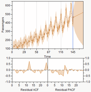
The Time Series platform begins with a plot of each times series by the time ID, or row number if no time ID is specified (Figure 14.2). The plot, like others in JMP, has features to resize the graph, highlight points with the cursor or brush tool, and label points. See the Using JMP for a discussion of these features.

Figure 14.2 Time Series Plot of Seriesg (Airline Passenger) Data

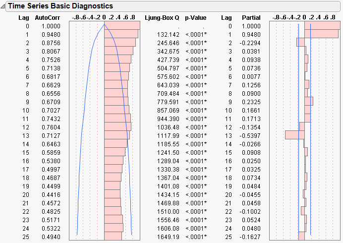
If you open Time Series Basic Diagnostic Tables, graphs of the autocorrelation and partial autocorrelation (Figure 14.3) of the time series are shown.

The platform popup menu, discussed next, also has fitting commands and options for displaying additional graphs and statistical tables.

Time Series Commands

The platform red triangle menu has the options described in the following sections.

Graph

The Time Series platform begins by showing a time series plot, like the one shown previously in Figure 14.2. The Graph command on the platform popup menu has a submenu of controls for the time series plot with the following commands.

Time Series Graph

hides or displays the time series graph.

Show Points

hides or displays the points in the time series graph.

Connecting Lines

hides or displays the lines connecting the points in the time series graph.

Mean Line

hides or displays a horizontal line in the time series graph that depicts the mean of the time series.

Autocorrelation

The Autocorrelation command alternately hides or displays the autocorrelation graph of the sample, often called the sample autocorrelation function. This graph describes the correlation between all the pairs of points in the time series with a given separation in time or lag. The autocorrelation for the kth lag is

where

is the mean of the N nonmissing points in the time series. The bars graphically depict the autocorrelations.

By definition, the first autocorrelation (lag 0) always has length 1. The curves show twice the large-lag standard error (± 2 standard errors), computed as

The autocorrelation plot for the Seriesg data is shown on the left in Figure 14.3. You can examine the autocorrelation and partial autocorrelations plots to determine whether the time series is stationary (meaning it has a fixed mean and standard deviation over time) and what model might be appropriate to fit the time series.

In addition, the Ljung-Box Q and p-values are shown for each lag. The Q-statistic is used to test whether a group of autocorrelations is significantly different from zero or to test that the residuals from a model can be distinguished from white-noise.

Partial Autocorrelation

The Partial Autocorrelation command alternately hides or displays the graph of the sample partial autocorrelations. The plot on the right in Figure 14.3 shows the partial autocorrelation function for the Seriesg data. The solid blue lines represent ± 2 standard errors for approximate 95% confidence limits, where the standard error is computed:

for all k

Figure 14.3 Autocorrelation and Partial Correlation Plots

Variogram

The Variogram command alternately displays or hides the graph of the variogram. The variogram measures the variance of the differences of points k lags apart and compares it to that for points one lag apart. The variogram is computed from the autocorrelations as

where rk is the autocorrelation at lag k. The plot on the left in Figure 14.4 shows the Variogram graph for the Seriesg data.

AR Coefficients

The AR Coefficients command alternately displays or hides the graph of the least squares estimates of the autoregressive (AR) coefficients. The definition of these coefficients is given below. These coefficients approximate those that you would obtain from fitting a high-order, purely autoregressive model. The right-hand graph in Figure 14.4 shows the AR coefficients for the Seriesg data.

Figure 14.4 Variogram Graph (left) and AR Coefficient Graph (right)

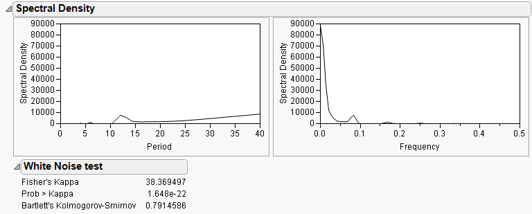
Spectral Density

The Spectral Density command alternately displays or hides the graphs of the spectral density as a function of period and frequency (Figure 14.5).

The least squares estimates of the coefficients of the Fourier series

and

where

are combined to form the periodogram

, which represents the intensity at frequency fi.

The periodogram is smoothed and scaled by 1/(4π) to form the spectral density.

The Fisher’s Kappa statistic tests the null hypothesis that the values in the series are drawn from a normal distribution with variance 1 against the alternative hypothesis that the series has some periodic component. Kappa is the ratio of the maximum value of the periodogram, I(fi), and its average value. The probability of observing a larger Kappa if the null hypothesis is true is given by

where q = N / 2 if N is even, q = (N - 1) / 2 if N is odd, and κ is the observed value of Kappa. The null hypothesis is rejected if this probability is less than the significance level α.

For q - 1 > 100, Bartlett’s Kolmogorov-Smirnov compares the normalized cumulative periodogram to the cumulative distribution function of the uniform distribution on the interval (0, 1). The test statistic equals the maximum absolute difference of the cumulative periodogram and the uniform CDF. If it exceeds

, then reject the hypothesis that the series comes from a normal distribution. The values a = 1.36 and a = 1.63 correspond to significance levels 5% and 1% respectively.

Figure 14.5 Spectral Density Plots

Save Spectral Density

Save Spectral Density creates a new table containing the spectral density and periodogram where the (i+1)th row corresponds to the frequency fi = i / N (that is, the ith harmonic of 1 / N).

The new data table has these columns:

Period

is the period of the ith harmonic, 1 / fi.

Frequency

is the frequency of the harmonic, fi.

Angular Frequency

is the angular frequency of the harmonic, 2πfi.

Sine

is the Fourier sine coefficients, ai.

Cosine

is the Fourier cosine coefficients, bi.

Periodogram

is the periodogram, I(fi).

Spectral Density

is the spectral density, a smoothed version of the periodogram.

Number of Forecast Periods

The Number of Forecast Periods command displays a dialog for you to reset the number of periods into the future that the fitted models will forecast. The initial value is set in the Time Series Launch dialog. All existing and future forecast results will show the new number of periods with this command.

Difference

Many time series do not exhibit a fixed mean. Such nonstationary series are not suitable for description by some time series models such as those with only autoregressive and moving average terms (ARMA models). However, these series can often be made stationary by differencing the values in the series. The differenced series is given by

where t is the time index and B is the backshift operator defined by Byt = yt-1.

The Difference command computes the differenced series and produces graphs of the autocorrelations and partial autocorrelations of the differenced series. These graphs can be used to determine if the differenced series is stationary.

Several of the time series models described in the next sections accommodate a differencing operation (the ARIMA, Seasonal ARIMA models, and some of the smoothing models). The Difference command is useful for determining the order of differencing that should be specified in these models.

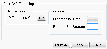
The Differencing Specification dialog appears in the report window when you select the Difference command. It allows you to specify the differencing operation you want to apply to the time series. Click Estimate to see the results of the differencing operation. The Specify Differencing dialog allows you to specify the Nonseasonal Differencing Order, d, the Seasonal Differencing Order, D, and the number of Periods Per Season, s. Selecting zero for the value of the differencing order is equivalent to no differencing of that kind.

The red triangle menu on the Difference plot has the following options:

Graph

controls the plot of the differenced series and behaves the same as those under the Time Series Graph menu.

Autocorrelation

alternately displays or hides the autocorrelation of the differenced series.

Partial Autocorrelation

alternately hides or displays the partial autocorrelations of differenced series.

Variogram

alternately hides or displays the variogram of the differenced series.

Save

appends the differenced series to the original data table. The leading d + sD elements are lost in the differencing process. They are represented as missing values in the saved series.

Modeling Reports

The time series modeling commands are used to fit theoretical models to the series and use the fitted model to predict (forecast) future values of the series. These commands also produce statistics and residuals that allow you to ascertain the adequacy of the model you have elected to use. You can select the modeling commands repeatedly. Each time you select a model, a report of the results of the fit and a forecast is added to the platform results.

The fit of each model begins with a dialog that lets you specify the details of the model being fit as well as how it will be fit. Each general class of models has its own dialog, as discussed in their respective sections. The models are fit by maximizing the likelihood function, using a Kalman filter to compute the likelihood function. The ARIMA, seasonal ARIMA, and smoothing models begin with the following report tables.

Model Comparison Table

Figure 14.6 shows the Model Comparison Report.

Figure 14.6 Model Comparison

The Model Comparison table summarizes the fit statistics for each model. You can use it to compare several models fitted to the same time series. Each row corresponds to a different model. The models are sorted by the AIC statistic. The Model Comparison table shown above summarizes the ARIMA models (1, 0, 0), (0, 0, 1), (1, 0, 1), and (1, 1, 1) respectively. Use the Report checkbox to show or hide the Model Report for a model.

The Model Comparison report has red-triangle menus for each model, with the following options:

Fit New

opens a window giving the settings of the model. You can change the settings to fit a different model.

Simulate Once

provides one simulation of the model out k time periods. The simulation is shown on the Model Comparison time series plot. To change k, use the Number of Forecast Periods option on the platform red-triangle menu.

Simulate More

provides the specified number of simulations of the model out k time periods. The simulations are shown on the Model Comparison time series plot. To change k, use the Number of Forecast Periods option on the platform red-triangle menu.

Remove Model Simulation

removes the simulations for the given model.

Remove All Simulation

removes the simulations for all models.

Generate Simulation

generates simulations for the given model, and stores the results in a data table. You specify the random seed, number of simulations, and the number of forecast periods.

Set Seed

is used to specify the seed for generating the next forecasts.

The Model Comparison report provides plots for a model when the Graph checkbox is selected. Figure 14.7 shows the plots for the ARIMA(1,1,1) model.

Figure 14.7 Model Plots

The top plot is a time series plot of the data, forecasts, and confidence limits. Below that are plots of the autocorrelation and partial autocorrelation functions.

Model Summary Table

Each model fit generates a Model Summary table, which summarizes the statistics of the fit. In the formulae below, n is the length of the series and k is the number of fitted parameters in the model.

is the number of degrees of freedom in the fit, n – k.

Sum of Squared Errors

is the sum of the squared residuals.

Variance Estimate

the unconditional sum of squares (SSE) divided by the number of degrees of freedom, SSE / (n – k). This is the sample estimate of the variance of the random shocks at, described in the section ARIMA Model.

Standard Deviation

is the square root of the variance estimate. This is a sample estimate of the standard deviation of at, the random shocks.

Akaike’s Information Criterion [AIC], Schwarz’s Bayesian Criterion [SBC or BIC]

Smaller values of these criteria indicate better fit. They are computed:

RSquare

RSquare is computed

where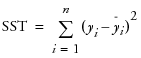

and

are the one-step-ahead forecasts, and

is the mean yi.

If the model fits the series badly, the model error sum of squares, SSE might be larger than the total sum of squares, SST and R2 will be negative.

RSquare Adj

The adjusted R2 is

MAPE

is the Mean Absolute Percentage Error, and is computed

MAE

is the Mean Absolute Error, and is computed

–2LogLikelihood

is minus two times the natural log of the likelihood function evaluated at the best-fit parameter estimates. Smaller values are better fits.

Stable

indicates whether the autoregressive operator is stable. That is, whether all the roots of

lie outside the unit circle.

Invertible

indicates whether the moving average operator is invertible. That is, whether all the roots of

lie outside the unit circle.

Note: The φ and θ operators are defined in the section ARIMA Model.

Parameter Estimates Table

There is a Parameter Estimates table for each selected fit, which gives the estimates for the time series model parameters. Each type of model has its own set of parameters. They are described in the sections on specific time series models. The Parameter Estimates table has these terms:

Term

lists the name of the parameter. These are described below for each model type. Some models contain an intercept or mean term. In those models, the related constant estimate is also shown. The definition of the constant estimate is given under the description of ARIMA models.

Factor (Seasonal ARIMA only)

lists the factor of the model that contains the parameter. This is only shown for multiplicative models. In the multiplicative seasonal models, Factor 1 is nonseasonal and Factor 2 is seasonal.

Lag (ARIMA and Seasonal ARIMA only)

lists the degree of the lag or backshift operator that is applied to the term to which the parameter is multiplied.

Estimate

lists the parameter estimates of the time series model.

Std Error

lists the estimates of the standard errors of the parameter estimates. They are used in constructing tests and confidence intervals.

t Ratio

lists the test statistics for the hypotheses that each parameter is zero. It is the ratio of the parameter estimate to its standard error. If the hypothesis is true, then this statistic has an approximate Student’s t-distribution. Looking for a t-ratio greater than 2 in absolute value is a common rule of thumb for judging significance because it approximates the 0.05 significance level.

Prob>|t|

lists the observed significance probability calculated from each t-ratio. It is the probability of getting, by chance alone, a t-ratio greater (in absolute value) than the computed value, given a true hypothesis. Often, a value below 0.05 (or sometimes 0.01) is interpreted as evidence that the parameter is significantly different from zero.

The Parameter Estimates table also gives the Constant Estimate, for models that contain an intercept or mean term. The definition of the constant estimate is given under ARIMA Model.

Forecast Plot

Each model has its own Forecast plot. The Forecast plot shows the values that the model predicts for the time series. It is divided by a vertical line into two regions. To the left of the separating line the one-step-ahead forecasts are shown overlaid with the input data points. To the right of the line are the future values forecast by the model and the confidence intervals for the forecasts.

You can control the number of forecast values by changing the setting of the Forecast Periods box in the platform launch dialog or by selecting Number of Forecast Periods from the Time Series drop-down menu. The data and confidence intervals can be toggled on and off using the Show Points and Show Confidence Interval commands on the model’s popup menu.

Residuals

The graphs under the residuals section of the output show the values of the residuals based on the fitted model. These are the actual values minus the one-step-ahead predicted values. In addition, the autocorrelation and partial autocorrelation of these residuals are shown. These can be used to determine whether the fitted model is adequate to describe the data. If it is, the points in the residual plot should be normally distributed about the zero line and the autocorrelation and partial autocorrelation of the residuals should not have any significant components for lags greater than zero.

Iteration History

The model parameter estimation is an iterative procedure by which the log-likelihood is maximized by adjusting the estimates of the parameters. The iteration history for each model you request shows the value of the objective function for each iteration. This can be useful for diagnosing problems with the fitting procedure. Attempting to fit a model which is poorly suited to the data can result in a large number of iterations that fail to converge on an optimum value for the likelihood. The Iteration History table shows the following quantities:

Iter

lists the iteration number.

Iteration History

lists the objective function value for each step.

Step

lists the type of iteration step.

Obj-Criterion

lists the norm of the gradient of the objective function.

Model Report Options

The title bar for each model you request has a popup menu, with the following options for that model:

Show Points

hides or shows the data points in the forecast graph.

Show Confidence Interval

hides or shows the confidence intervals in the forecast graph.

Save Columns

creates a new data table with columns representing the results of the model.

Save Prediction Formula

saves the data and prediction formula to a new data table.

Create SAS Job

creates SAS code that duplicates the model analysis in SAS.

Submit to SAS

submits code to SAS that duplicates the model analysis. If you are not connected to a SAS server, prompts guide you through the connection process.

Residual Statistics

controls which displays of residual statistics are shown for the model. These displays are described in the section Time Series Commands; however, they are applied to the residual series.

ARIMA Model

An AutoRegressive Integrated Moving Average (ARIMA) model predicts future values of a time series by a linear combination of its past values and a series of errors (also known as random shocks or innovations). The ARIMA command performs a maximum likelihood fit of the specified ARIMA model to the time series.

For a response series

, the general form for the ARIMA model is:

where

t is the time index

B is the backshift operator defined as

is the response series after differencing

μ is the intercept or mean term.

and

, respectively, the autoregressive operator and the moving average operator and are written

and

are the sequence of random shocks.

The

are assumed to be independent and normally distributed with mean zero and constant variance.

The model can be rewritten as

where the constant estimate δ is given by the relation

The ARIMA command displays the Specify ARIMA Model dialog, which allows you to specify the ARIMA model you want to fit. The results appear when you click Estimate.

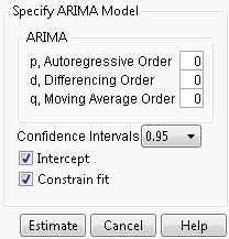
Use the Specify ARIMA Model dialog for the following three orders that can be specified for an ARIMA model:

1. The Autoregressive Order is the order (p) of the polynomial

operator.

2. The Differencing Order is the order (d) of the differencing operator.

3. The Moving Average Order is the order (q) of the differencing operator

4. An ARIMA model is commonly denoted ARIMA(p,d,q). If any of p,d, or q are zero, the corresponding letters are often dropped. For example, if p and d are zero, then model would be denoted MA(q).

The Confidence Intervals box allows you to set the confidence level between 0 and 1 for the forecast confidence bands. The Intercept check box determines whether the intercept term μ will be part of the model. If the Constrain fit check box is checked, the fitting procedure will constrain the autoregressive parameters to always remain within the stable region and the moving average parameters within the invertible region. You might want to uncheck this box if the fitter is having difficulty finding the true optimum or if you want to speed up the fit. You can check the Model Summary table to see if the resulting fitted model is stable and invertible.

Seasonal ARIMA

In the case of Seasonal ARIMA modeling, the differencing, autoregressive, and moving average operators are the product of seasonal and nonseasonal polynomials:

where s is the number of periods in a season. The first index on the coefficients is the factor number (1 indicates nonseasonal, 2 indicates seasonal) and the second is the lag of the term.

The Seasonal ARIMA dialog appears when you select the Seasonal ARIMA command. It has the same elements as the ARIMA dialog and adds elements for specifying the seasonal autoregressive order (P), seasonal differencing order (D), and seasonal moving average order (Q). Also, the Periods Per Season box lets you specify the number of periods per season (s). The seasonal ARIMA models are denoted as Seasonal ARIMA(p,d,q)(P,D,Q)s.

ARIMA Model Group

The ARIMA Model Group option on the platform red-triangle menu allows the user to fit a range of ARIMA or Seasonal ARIMA models by specifying the range of orders. Figure 14.8 shows the dialog.

Figure 14.8 ARIMA Group

Transfer Functions

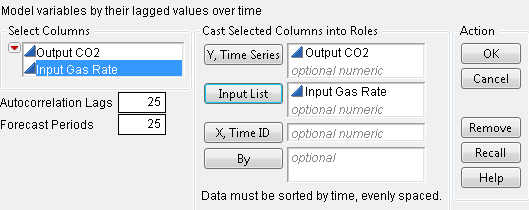
This example analyzes the gas furnace data (seriesJ.jmp) from Box and Jenkins. To begin the analysis, select Input Gas Rate as the Input List and Output CO2 as the Y, Time Series. The launch dialog should appear as in Figure 14.9.

Figure 14.9 Series J Launch Dialog

When you click OK, the report in Figure 14.10 appears.

Report and Menu Structure

This preliminary report shows diagnostic information and groups the analysis in two main parts. The first part, under Time Series Output CO2, contains analyses of the output series, while the Input Time Series Panel, contains analyses on the input series. The latter may include more than one series.

Figure 14.10 Series J Report

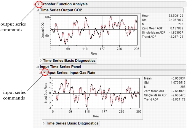
Each report section has its own set of commands. For the output (top) series, the commands are accessible from the red triangle on the outermost outline bar (Transfer Function Analysis). For the input (bottom) series, the red triangle is located on the inner outline bar (Input Series: Input Gas Rate).

Figure 14.11 shows these two command sets. Note their organization. Both start with a Graph command. The next set of commands are for exploration. The third set is for model building. The fourth set includes functions that control the platform.

Figure 14.11 Output and Input Series Menus

Diagnostics

Both parts give basic diagnostics, including the sample mean (Mean), sample standard deviation (Std), and series length (N).

In addition, the platform tests for stationarity using Augmented Dickey-Fuller (ADF) tests.

Zero Mean ADF

tests against a random walk with zero mean, i.e.

Single Mean ADF

tests against a random walk with a non-zero mean, i.e.

Trend ADF

tests against a random walk with a non-zero mean and a linear trend, i.e.

Basic diagnostics also include the autocorrelation and partial autocorrelation functions, as well as the Ljung-Box Q-statistic and p-values, found under the Time Series Basic Diagnostics outline node.

The Cross Correlation command adds a cross-correlation plot to the report. The length of the plot is twice that of an autocorrelation plot, or

Figure 14.12 Cross Correlation Plot

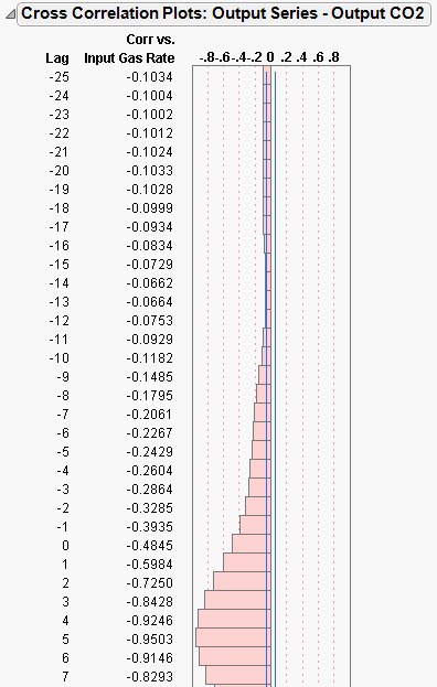
The plot includes plots of the output series versus all input series, in both numerical and graphical forms. The blue lines indicate standard errors for the statistics.

Model Building

Building a transfer function model is quite similar to building an ARIMA model, in that it is an iterative process of exploring, fitting, and comparing.

Before building a model and during the data exploration process, it is sometimes useful to prewhiten the data. This means find an adequate model for the input series, apply the model to the output, and get residuals from both series. Compute cross-correlations from residual series and identify the proper orders for the transfer function polynomials.

To prewhiten the input series, select the Prewhitening command. This brings up a dialog similar to the ARIMA dialog where you specify a stochastic model for the input series. For our SeriesJ example, we use an ARMA(2,2) prewhitening model, as shown in Figure 14.13.

Figure 14.13 Prewhitening Dialog

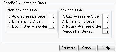
Click Estimate to reveal the Prewhitening plot.

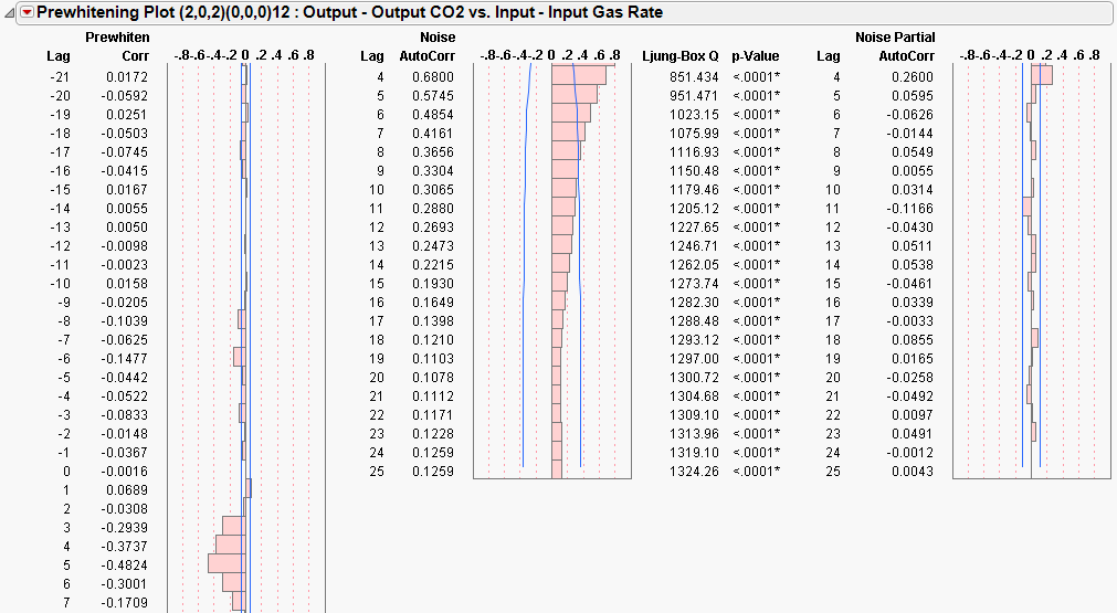
Patterns in these plots suggest terms in the transfer function model.

Transfer Function Model

A typical transfer function model with m inputs can be represented as

where

Yt denotes the output series

X1 to Xm denote m input series

et represents the noise series

X1, t–d1 indicates the series X1 is indexed by t with a d1-step lag

μ represents the mean level of the model

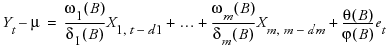
ϕ(B) and θ(B) represent autoregressive and moving average polynomials from an ARIMA model

ωk(B) and δk(B) represent numerator and denominator factors (or polynomials) for individual transfer functions, with k representing an index for the 1 to m individual inputs.

Each polynomial in the above model can contain two parts, either nonseasonal, seasonal, or a product of the two as in seasonal ARIMA. When specifying a model, leave the default 0 for any part that you do not want in the model.

Select Transfer Function to bring up the model specification dialog.

Figure 14.14 Transfer Function Specification Dialog

The dialog consists of several parts.

Noise Series Orders

contains specifications for the noise series. Lowercase letters are coefficients for non-seasonal polynomials, and uppercase letters for seasonal ones.

Choose Inputs

lets you select the input series for the model.

Input Series Orders

specifies polynomials related to the input series.The first three orders deal with non-seasonal polynomials. The next four are for seasonal polynomials. The final is for an input lag.

In addition, there are three options that control model fitting.

Intercept

specifies whether μ is zero or not.

Alternative Parameterization

specifies whether the general regression coefficient is factored out of the numerator polynomials.

Constrain Fit

toggles constraining of the AR and MA coefficients.

Forecast Periods

specifies the number of forecasting periods for forecasting.

Using the information from prewhitening, we specify the model as shown in Figure 14.14.

Model Reports

The analysis report is titled Transfer Function Model and is indexed sequentially. Results for the Series J example are shown in Figure 14.15.

Figure 14.15 Series J Transfer Function Reports

Model Summary

gathers information that is useful for comparing models.

Parameter Estimates

shows the parameter estimates and is similar to the ARIMA version. In addition, the Variable column shows the correspondence between series names and parameters. The table is followed by the formula of the model. Note the notation B is for the backshift operator.

Residuals, Iteration History

are the same as their ARIMA counterparts.

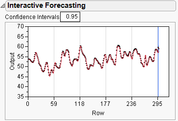
Interactive Forecasting

provides a forecasting graph based on a specified confidence interval. The functionality changes based on the number entered in the Forecast Periods box.

If the number of Forecast Periods is less than or equal to the Input Lag, the forecasting box shows the forecast for the number of periods. A confidence interval around the prediction is shown in blue, and this confidence interval can be changed by entering a number in the Confidence Interval box above the graph.

If the number of forecast periods is larger than the number of lags (say, eight in our example), the presentation is a little different.

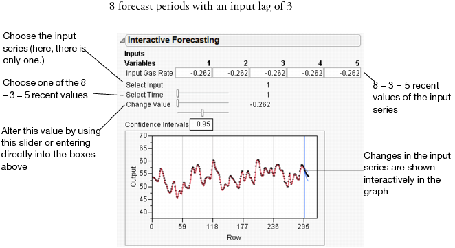
Here, you manipulate lagged values of the series by entering values into the edit boxes next to the series, or by manipulating the sliders. As before, the confidence interval can also be changed. The results of your changes are reflected in real time in the Interactive Forecasting graph.

The following commands are available from the report drop-down menu.

Save Columns

creates a new data table containing the input and output series, a time column, predicted output with standard errors, residuals, and 95% confidence limits.

Create SAS Job

creates PROC ARIMA code that can reproduce this model.

Submit to SAS

submits PROC ARIMA code to SAS that reproduces the model.

Model Comparison Table

The model comparison table works like its ARIMA counterpart by accumulating statistics on the models you specify.

Fitting Notes

A regression model with serially correlated errors can be specified by including regressors in the model and not specifying any polynomial orders.

Intervention analysis can also be conducted, but prewhitening is no longer meaningful.

Currently, the transfer function model platform has limited capability of supporting missing values.

Smoothing Models

JMP offers a variety of smoothing techniques.

Smoothing models represent the evolution of a time series by the model:

where

is the time-varying mean term,

is the time-varying slope term,

is one of the s time-varying seasonal terms,

are the random shocks.

Models without a trend have

and nonseasonal models have

. The estimators for these time-varying terms are

smoothed level that estimates

is a smoothed trend that estimates

for

are the estimates of the

Each smoothing model defines a set of recursive smoothing equations that describes the evolution of these estimators. The smoothing equations are written in terms of model parameters called smoothing weights. They are

α, the level smoothing weight

γ, the trend smoothing weight

ϕ, the trend damping weight

δ, the seasonal smoothing weight.

While these parameters enter each model in a different way (or not at all), they have the common property that larger weights give more influence to recent data while smaller weights give less influence to recent data.

Each smoothing model has an ARIMA model equivalent. You may not be able to specify the equivalent ARIMA model using the ARIMA command because some smoothing models intrinsically constrain the ARIMA model parameters in ways the ARIMA command will not allow.

Simple Moving Average

A simple moving average model (SMA) produces forecasted values that are equal to the average of consecutive observations in a time window. The forecasts can be uncentered or centered in the time window.

To fit a simple moving average model, select Smoothing > Simple Moving Average. A window appears with the following options:

Enter smoothing window width

Enter the width of the smoothing window.

Centered

Choose whether to center the forecasted values.

The Simple Moving Average report shows a time plot of the data and the fitted model. The red triangle menu has the following options:

Add Model

Select this option to fit another model. When additional models are fit, the model is added to the time plot of the data.

Save to Data Table

Saves the original data, and forecasts of all moving average models.

Show Points

Shows or hides the points on the plot.

Connecting Lines

Shows or hides the lines on the plot.

Smoothing Model Dialog

The Smoothing Model dialog appears in the report window when you select one of the smoothing model commands.

The Confidence Intervals popup list allows you to set the confidence level for the forecast confidence bands. The dialogs for seasonal smoothing models include a Periods Per Season box for setting the number of periods in a season. The Constraints popup list lets you to specify what type of constraint you want to enforce on the smoothing weights during the fit. The constraints are:

Zero To One

keeps the values of the smoothing weights in the range zero to one.

Unconstrained

allows the parameters to range freely.

Stable Invertible

constrains the parameters such that the equivalent ARIMA model is stable and invertible.

Custom

expands the dialog to allow you to set constraints on individual smoothing weights. Each smoothing weight can be Bounded, Fixed, or Unconstrained as determined by the setting of the popup menu next to the weight’s name. When entering values for fixed or bounded weights, the values can be positive or negative real numbers.

The example shown here has the Level weight (α) fixed at a value of 0.3 and the Trend weight (γ) bounded by 0.1 and 0.8. In this case, the value of the Trend weight is allowed to move within the range 0.1 to 0.8 while the Level weight is held at 0.3. Note that you can specify all the smoothing weights in advance by using these custom constraints. In that case, none of the weights would be estimated from the data although forecasts and residuals would still be computed. When you click Estimate, the results of the fit appear in place of the dialog.

Simple Exponential Smoothing

The model for simple exponential smoothing is

The smoothing equation, Lt = αyt + (1 – α)Lt-1, is defined in terms of a single smoothing weight α. This model is equivalent to an ARIMA(0, 1, 1) model where