
Overview of the Life Distribution Platform
Life data analysis, or life distribution analysis, is the process of modeling the lifespan of a product, component, or system to predict lifetime or time to failure. For example, you can observe failure rates over time to predict when a computer component might fail. This technique enables you to compare materials and manufacturing processes for the product, allowing you to increase the quality and reliability of the product. Decisions on warranty periods and advertising claims can also be more accurate.
With the Life Distribution platform, you can analyze censored data in which some time observations are unknown. And if there are potentially multiple causes of failure, you can analyze the competing causes to estimate which cause is more influential.
You can use the Reliability Test Plan and Reliability Demonstration calculators to choose the appropriate sample sizes for reliability studies. These calculators are found at DOE > Sample Size and Power. See the Prospective Sample Size and Power chapter in the Design of Experiments Guide.
Example of the Life Distribution Platform
Suppose you have failure times for 70 engine fans, with some of the failure times censored. You want to fit a distribution to the failure times and then estimate various measurements of reliability.
1. Select Help > Sample Data Library and open Reliability/Fan.jmp.
2. Select Analyze > Reliability and Survival > Life Distribution.
3. Select Time and click Y, Time to Event.
4. Select Censor and click Censor.
5. Click OK.
The Life Distribution report window appears.
6. In the Compare Distribution report, select Lognormal distribution and the corresponding Scale radio button.
A probability plot appears in the report window (Figure 3.2).
Figure 3.2 Probability Plot
In the probability plot, the data points generally fall along the red line, indicating that the lognormal fit is reasonable.
Below the Compare Distributions report, the Statistics report appears (Figure 3.3). This report provides a Model Comparison report, nonparametric and parametric estimates, profilers, and more.
Figure 3.3 Statistics Report

The parameter estimates for the lognormal distribution are provided. The profilers are useful for visualizing the fitted distribution and for estimating probabilities and quantiles. For example, the Quantile Profiler indicates that the estimated median time to failure is 25,418.67 hours.
Launch the Life Distribution Platform
Launch the Life Distribution platform by selecting Analyze > Reliability and Survival > Life Distribution.
Figure 3.4 Life Distribution Launch Window

Launch Window Tabs
The launch window includes two tabs:
• The Life Distribution tab models ungrouped data. The following types of reports can result:
‒ The Life Distribution report appears when you do not specify a Failure Cause role. From this report, you can compare common distributions and examine statistics. See “Life Distribution Report”.
‒ The Weibayes report appears when you have zero failures in your data. See “Weibayes Report”.
‒ The Competing Cause report appears when you specify a Failure Cause role. In addition to the features in the Life Distribution report, you can also compare individual failure causes. See “Competing Cause Report”.
Note: You can examine Fixed Parameter and Bayesian models in the Life Distribution and Competing Cause reports.
• The Compare Groups tab enables you to specify a Grouping variable. The Compare Groups report compares different groups using a single specified distribution. For example, you might compare Weibull fits for components grouped by supplier. In contrast, the Life Distribution tab compares several fitted distributions for a single group. See “Life Distribution - Compare Groups Report”.
Launch Window Options
The launch window contains the following options:
Y, Time to Event
The time to event (such as the time to failure) or time to right censoring. For interval censoring, specify two Y variables, where one Y variable gives the lower limit and the other Y variable gives the upper limit for each unit. For details about censoring, see “Event Plot”.
Grouping
(Appears only in the Compare Groups tab.) A column containing the groups that you want to compare. For an example, see “Examine the Same Distribution across Groups”.
Censor
A column that identifies right-censored observations. Select the value that identifies right-censored observations from the Censor Code menu beneath the Select Columns list. The Censor column is used only when one Y is entered.
Failure Cause
A column that contains multiple failure causes. If a Failure Cause column is selected, then a section is added to the window:
‒ Check boxes appear that allow the failure mode to use ZI distributions, TH distributions, DS distributions, fixed parameter models or Bayesian models for the analysis.
‒ Distribution specifies the initial distribution to fit for each failure cause. Select one distribution to fit for all causes; select Individual Best to let the platform automatically choose the best fit for each cause; or select Manual Pick to manually choose the distribution to fit for each failure cause after JMP creates the Life Distribution report. You can also change the distribution fits in the Life Distribution report itself.
‒ Comparison Criterion is an option that appears only when you choose the Individual Best distribution fit. Select the method by which JMP chooses the best distribution: Corrected Akaike Information Criterion (AICc), Bayesian Information Criterion (BIC), or twice the negative log-likelihood (-2*LogLikelihood). For more details, see the Statistical Details appendix in the Fitting Linear Models book. You can change the method later in the Model Comparisons report. See “Model Comparisons” for details.
‒ Censor Indicator in Failure Cause Column identifies the indicator used in the Failure Cause column for observations that did not fail. To specify such an indicator, select this option and then enter the indicator in the box that appears.
See Meeker and Escobar (1998, chap. 15) for a discussion of multiple failure causes. “Omit Competing Causes” illustrates how to analyze multiple causes.
Freq
A column that contains frequencies or observation counts when the information in a row represents multiple units. If the value in a row is 0 or a positive number, then the value represents the frequencies or counts of observations for that row.
Label
A column that contains identifiers other than the row number. These labels appear on the y axis in the event plot.
By
An optional variable whose levels define rows used to create separate models.
Censor Code
After selecting the Censor column, select the value that designates right-censored observations from the list. Missing values are excluded from the analysis. JMP attempts to detect the censor code and display it in the list.
Select Confidence Interval Method
Defines the method used for computing confidence intervals for the parameters. The default is Wald, but you can select Likelihood instead. However, all confidence intervals provided in the profilers are based on the Wald method. This is done to reduce computation time. For more information, refer to “Estimation and Confidence Intervals”.
Failure Distribution by Cause
Appears only in the Life Distribution tab when a Cause is specified. Specify which families of distributions should be available to model the life distributions for individual causes. Select an initial distribution, Individual Best, or Manual Pick from the Distribution menu. For details, see “Failure Cause”.
Life Distribution Report
Tip: If you find that the report window is too long, select Tabbed Report from the red triangle menu.
If you have not selected a Failure Cause in the launch window, you will see the Life Distribution report. Use this report to analyze lifetime data where some time observations might be censored. The Life Distribution report contains the following content and options:
Figure 3.5 Example of the Life Distribution Report for Fan.jmp

Event Plot
Click the Event Plot disclosure icon to see a plot of the failure or censoring times. For each row in the data table, the Event Plot shows a horizontal line indicating whether the units in the row have been censored. When units have been censored, the line indicates the nature of the censoring. The censoring information is conveyed as follows:
• The time period when the units in the row are known to be functioning is indicated with a solid line.
• The time period when it is not known if the units in the row are functioning is indicated with a dashed line.
• The line terminates once the units in the row are known to have failed.
Single Time to Event Column
In the Fan.jmp sample data table there is a single Time column indicating failure time. When the failure time is unknown, the value Censored is recorded in the Censor column. All censored units are assumed to be right-censored. Figure 3.6 shows the Event Plot for this data.
Note: To construct the plot in Figure 3.6, select Help > Sample Data Library and open Reliability/Fan.jmp. Click the green triangle next to the Life Distribution - Exponential script. Click the Event Plot disclosure icon.
Figure 3.6 Event Plot for Right-Censored Data
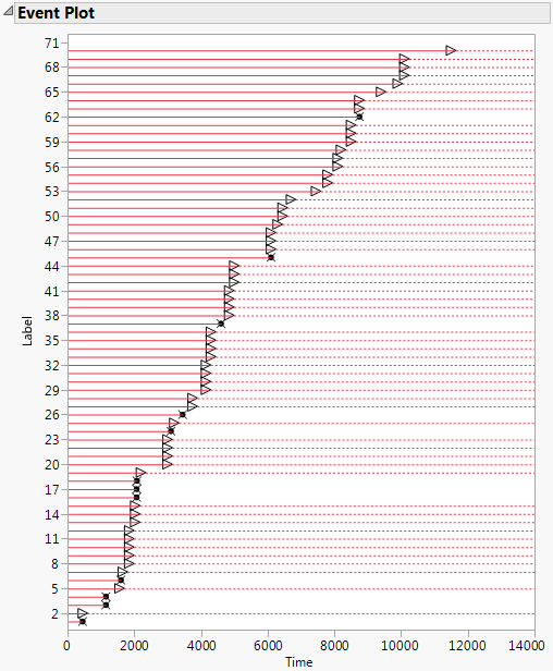
The unit in row 3 failed at Time 1150. Its lifetime is represented by a solid horizontal line that ends at Time 1150. The failure time is marked with an “x”.
The unit in row 5 is right censored. It was last know to be functioning at Time 1560. The time period during which the unit is known to be functioning is represented by a solid horizontal line that ends at Time 1560. At Time 1560, a right arrow is plotted. The line continues as a dashed line, indicating that the failure time is unknown, but greater than 1560.
Two Time to Event Columns
In the Censor Labels.jmp sample data table, there are two columns, Start Time and End Time. Start Time indicates when units in a row were last known to be functioning. End Time indicates when units in that row were first known to have failed.
The Start Time and End Time values indicate the following about the units:
• Units in rows 1 and 2 are left censored. They were known to fail before the time in the End Time column, but their exact failure times are unknown.
• Units in rows 3 and 4 are right censored. They were known to be last functioning at the time in the Start Time column, but their failure times are unknown.
• Units in rows 5 and 6 are interval censored. They were known to fail within the interval defined by the Start Time and End Time.
• Units in rows 7 and 8 are not censored. Their failure times are given by the values in the Start Time and End Time columns, which are identical.
Figure 3.7 shows the Event Plot for this data.
Note: To construct the plot in Figure 3.7, select Help > Sample Data Library and open Censor Labels.jmp. Click the green triangle next to the Life Distribution script.
Figure 3.7 Event Plot for Mixed-Censored Data

The various types of censoring are represented as follows:
• The pattern  indicates right censoring. The unit failed after its last inspection.
• The pattern  indicates left censoring. The unit failed after being put on test and prior to the indicated time, but it is not known when it was last functioning.
• The pattern  indicates that the unit failed during the time interval marked by the two arrow heads.
• The pattern  indicates no censoring. The unit failed at the time marked by the x.
Compare Distributions
The Compare Distributions report lets you fit and compare different failure time distributions. Two lists appear:
Distribution
Select a distribution for the response. Different distributions appear based on characteristics of the data. For details about which distributions are available, see “Available Parametric Distributions”.
Scale
Select a scale for the probability axis. The probability scale corresponds to the distribution listed to the left of the Scale button. Using this scale, the fitted model is represented by a line. Suppose that you fit a given distribution and then scale the axis using that distribution. If the points generally fall along a line, this indicates that the distribution provides a reasonable fit.
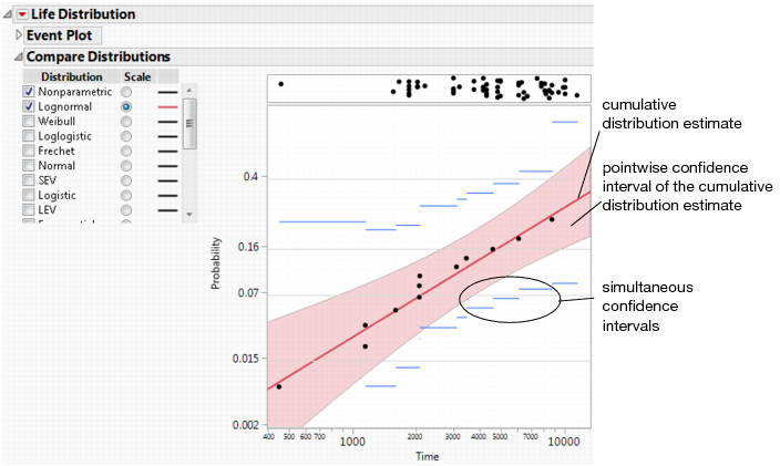
The default plot shows the nonparametric estimates (Kaplan-Meier-Turnbull) for the uncensored data values and their confidence intervals. The confidence intervals are indicated by horizontal blue lines.
By default, there is a panel at the top of the plot that displays times of right-censored observations. The Show Markers for Right Censored Observations preference determines whether this panel appears by default. You can change this preference in Preferences > Platforms > Life Distribution.
For each distribution that you select, the Compare Distributions report is updated to show the following:
• the estimated cumulative distribution curve, which appears on the probability plot
• a shaded region that indicates confidence intervals for the cumulative distribution
• a Distribution Profiler that shows the cumulative probability of failure for a given period of time
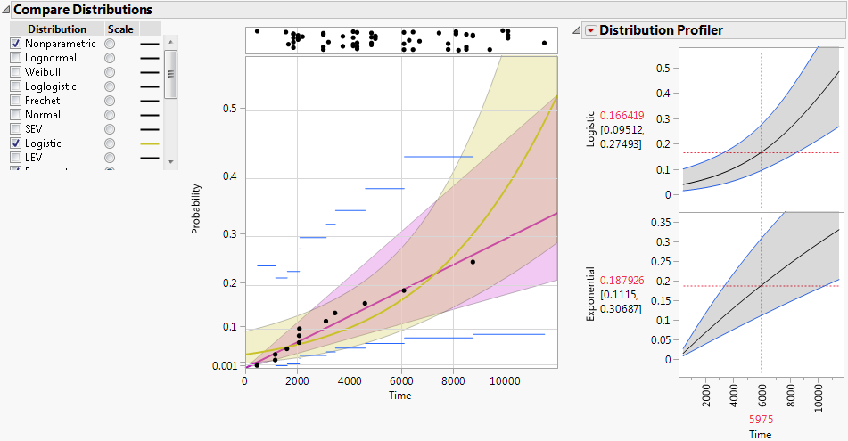
Figure 3.8 shows an example of the Compare Distributions report. The Logistic (yellow) and Exponential (magenta) distributions are shown. The plot is scaled using the Exponential distribution.
Figure 3.8 Compare Distributions Report and Distribution Profiler
Available Parametric Distributions
This section addresses the distributions available in the Compare Distributions report.
Note: Distributions for the Competing Cause report are covered in “Available Distributions for Competing Cause Compare Distributions Reports”.
The available distributions are listed and described in detail in “Parametric Distributions”. There are four major groupings of parametric distributions:
You can restrict which distributions are available by default by deselecting the ones that you do not want to appear. Select File > Preferences > Platforms > Life Distribution. The distributions listed include the Threshold, Defective Subpopulation, Zero-Inflated, LogGenGamma, and GenGamma distributions. By default, all of the distributions are checked and available.
The rules that determine which distributions appear in the Compare Distributions panel depend on the particular implementation. As a general guide, distributions are available if they are not disabled in Preferences and if they are appropriate in the given situation.
Basic Failure-Time Distributions
The basic failure-time distributions are available whenever all failure times are positive. They include the following:
• Lognormal
• Weibull
• Loglogistic
• Fréchet
• Normal
• SEV
• Logistic
• LEV
• Exponential
• LogGenGamma
• GenGamma
Note: When there are negative or zero failure times, only the Normal, SEV, Logistic, LEV, and LogGenGemma are available.
Threshold Distributions
The threshold (TH) distributions are always available. Threshold distributions are log-location-scale distributions with threshold parameters. The threshold parameter shifts the distribution away from 0. These distributions assume that all units survive until the threshold value. Threshold distributions are useful for fitting moderate to heavily shifted distributions. The threshold distributions are the following:
• TH Lognormal
• TH Weibull
• TH Loglogistic
• TH Fréchet
Defective Subpopulation Distributions
The defective subpopulation (DS) distributions are available when all failure times are positive. These distributions are useful when only a fraction of the population has a particular defect leading to failure. Use the DS distribution options to model failures that occur on only a subpopulation. The DS distributions are the following:
• DS Lognormal
• DS Weibull
• DS Loglogistic
• DS Fréchet
Zero-Inflated Distributions
When the time-to-event data contain zero as the minimum value in the Life Distribution platform, the following zero-inflated distributions are available:
• Zero-Inflated Lognormal (ZI Lognormal)
• Zero-Inflated Weibull (ZI Weibull)
• Zero-Inflated Loglogistic (ZI Loglogistic)
• Zero-Inflated Fréchet (ZI Fréchet)
Zero-inflated distributions are used when some proportion of units fail at time zero. When the data contain more zeros than expected by a standard model, the number of zeros is inflated.
Zero-Failure Data
In the case of zero-failure data, none of the above distributions are available by default. However, you can uncheck the preference called Weibayes Only for Zero Failure Data. This enables you to obtain Bayesian fits for those distributions where the Bayesian Estimate option is available. See “Weibayes Only for Zero Failure Data”.
Parametric Distributions That Allow Bayesian Estimation
Bayesian estimation is available for the following parametric distributions:
• Lognormal
• Weibull
• Loglogistic
• Fréchet
• Normal
• SEV
• Logistic
• LEV
A list of distributions that are available as priors for hyperparameters of these distributions is given in “Prior Distributions for Bayesian Estimation”.
Life Distribution: Statistics
The Statistics report includes the following sub-reports:
• “Parametric Estimate - <Distribution Name>” (one report appears for each distribution that you select in the Compare Distributions report)
Model Comparisons
The Model Comparisons report provides the AICc, -2*LogLikelihood, and BIC statistics for each fitted distribution. Smaller values of each of these statistics indicate a better fit. For more details on these statistics, see the Statistical Details appendix in the Fitting Linear Models book.
Initially, the rows are sorted by AICc. To change the statistic used to sort the report, select Comparison Criterion from the Life Distribution red triangle menu. See “Life Distribution Report Options” for details about this option.
Summary of Data
The Summary of Data report shows the total number of units observed, the number of uncensored units, and the numbers of right-censored, left-censored, and interval-censored units.
Nonparametric Estimate
The Nonparametric Estimate report shows nonparametric estimates for each observation. For right-censored data specified as a single Time to Event column, the report gives the following:
Midpoint Estimate
Midpoint-adjusted Kaplan-Meier estimates.
Lower 95%, Upper 95%
Pointwise 95% confidence intervals. You can change the confidence level by selecting Change Confidence Level from the report options.
Simultaneous Lower 95% (Nair), Simultaneous Upper 95% (Nair)
Simultaneous 95% confidence intervals. You can change the confidence level by selecting Change Confidence Level from the report options. See Nair (1984) and Meeker and Escobar (1998).
Kaplan-Meier Estimate
Standard Kaplan-Meier estimates.
If failure times are represented by two Time to Event columns, the report gives Turnbull estimates (in a column called Estimate), pointwise confidence intervals, and simultaneous confidence intervals (Nair).
See “Nonparametric Fit” for more information about nonparametric estimates.
Parametric Estimate - <Distribution Name>
A report called Parametric Estimate - <Distribution Name> appears for each distribution that is fit. The report gives the distribution’s parameter estimates, their standard errors, and confidence intervals. The criteria that appear in the Model Comparisons report are shown under Criterion.
Note: Whenever an estimate of the mean is provided, its confidence interval is computed as a Wald interval even if you select Likelihood as the Confidence Interval Method in the launch window. In this case, the notation Mean (Wald CI) appears in the Parameter column to indicate that the confidence interval for the mean is a Wald interval.
For details about how the distributions are parametrized, see “Parametric Distributions”.
The Parametric Estimate report contains the following reports:
• Additional reports can be added by selecting report options from the Parametric Estimate red triangle menu. These include the Fix Parameter, Bayesian Estimates, Custom Estimation (Estimate Probability, Estimate Quantile), and Mean Remaining Life reports. For details, see “Parametric Estimate Options”.
Covariance Matrix
For each distribution, the Covariance Matrix report shows the covariance matrix for the estimates.
Profilers
Four types of profilers appear for each distribution:
• The Distribution Profiler shows cumulative failure probability as a function of time.
• The Quantile Profiler shows failure time as a function of cumulative probability.
• The Hazard Profiler shows the hazard rate as a function of time.
• The Density Profiler shows the density function for the distribution.
The profilers contain the following red triangle options:
Confidence Intervals
The Distribution, Quantile, and Hazard profilers show Wald-based confidence curves for the plotted functions. This option shows or hides the confidence curves.
Reset Factor Grid
Displays a window for each factor allowing you to enter a specific value for the factor’s current setting, to lock that setting, and to control aspects of the grid. For details, see the Profiler chapter in the Profilers book.
Factor Settings
Provides a menu that consists of several options. For details, see the Profiler chapter in the Profilers book.
Note: The confidence intervals provided in the profilers are based on the Wald method even if the Likelihood Confidence Interval Method is selected in the launch window. This is done to reduce computation time.
Parametric Estimate Options
The Parametric Estimate red triangle menu has the following options:
Save Probability Estimates
Saves the estimated failure probabilities and confidence intervals to the data table.
Save Quantile Estimates
Saves the estimated quantiles and confidence intervals to the data table.
Save Hazard Estimates
Saves the estimated hazard values and confidence intervals to the data table.
Show Likelihood Contour
Shows or hides a contour plot of the log-likelihood function. If you have selected the Weibull distribution, a second contour plot appears for the alpha-beta parameterization. This option is available only for distributions with two parameters.
Show Likelihood Profiler
Shows or hides a profiler of the log-likelihood function. This option is not available for the threshold (TH) distributions.
Fix Parameter
Opens a report where you can specify the value of parameters. Enter your fixed parameter values, select the appropriate check box, and then click Update. JMP re-estimates the other parameters, covariances, and profilers based on the new parameters, and shows them in the Fix Parameter report. For an example in a competing cause situation, see “Specify a Fixed Parameter Model as a Distribution for a Cause”.
For the Weibull distribution, the Fix Parameter option lets you select the Weibayes method. For an example, see “Weibayes Estimates”. The Weibayes option is not available for interval-censored data.
Bayesian Estimates
Performs Bayesian estimation of parameters for certain distributions based on three methods of specifying prior distributions (Location and Scale Priors, Quantile and Parameter Priors, and Failure Probability Priors). See “Bayesian Estimation - <Distribution Name>”. This option is available only for the following distributions: Lognormal, Weibull, Loglogistic, Fréchet, Normal, SEV, Logistic, LEV.
Custom Estimation
Provides calculators that enable you to predict failure probabilities, survival probabilities, and quantiles for specific time and failure probability values. Each calculated quantity includes confidence intervals, which can be two-sided or one-sided (in either direction). Two reports appear: Estimate Probability and Estimate Quantile. See “Custom Estimation”.
Mean Remaining Life
Provides a calculator that enables you to estimate the mean remaining life of a unit. In the Mean Remaining Life Calculator, enter a Time and press Enter to see the estimate. Click the plus sign to enter additional times. This calculator is available for the following distributions: Lognormal, Weibull, Loglogistic, Fréchet, Normal, SEV, Logistic, LEV, and Exponential.
Bayesian Estimation - <Distribution Name>
For certain distributions, the platform fits Bayesian models. This is done using a Markov Chain Monte Carlo (MCMC) algorithm. More specifically, Bayesian estimation uses an independence chain sampler variation of the Metropolis-Hastings algorithm. See Robert and Casella (2004).
From the Parametric Estimate - <Distribution Name> report outline, select Bayesian Estimates. This opens an outline called Bayesian Estimation - <Distribution Name>. The initial report is a control panel where you can specify the parameters for the priors and control aspects of the simulation.
The workflow is as follows:
• Select a prior specification method from the Bayesian Estimation red triangle menu and set values for the parameters of the priors. See “Bayesian Estimation Red Triangle Options”.
• Specify the simulation options. See “Bayesian Estimates - Result <N>”.
• Select Fit Model to fit a model. See “Bayesian Estimates - Result <N>”.
Bayesian Estimation Red Triangle Options
You can choose from the following prior specification methods in the Bayesian Estimation red triangle menu:
Location and Scale Priors
Enables you to specify hyperparameters for prior distributions on generic parameters (location and scale parameters). Select the Prior Distribution red triangle menu to select a distribution for each parameter. You can enter new values for the hyperparameters of the priors. The initial values that are provided are estimates consistent with the MLEs. For details, see “Prior Distributions for Bayesian Estimation”.
Quantile and Parameter Priors
Enables you to specify prior information about a quantile and the scale parameter (or Weibull β if the parametric fit is Weibull). The quantile is defined by the value next to Probability. The default Probability value is 0.10, but you can specify a value that corresponds to the quantile of interest. Specify information about the prior information in terms of Lower and Upper 99% limits on the range of each prior distribution. See Meeker and Escobar, 1998. The initial values that are provided are estimates consistent with the MLEs. For details, see “Prior Distributions for Bayesian Estimation”.
Failure Probability Priors
Enables you to specify prior information about failure probabilities at two distinct time points. You can specify the two time points. The prior distribution for each time point is Beta. You can specify the prior distributions using either of two synchronized approaches:
1. Specify failure probability by estimates and error percentages. The prior information for each Beta prior distribution can be specified using a probability estimate and an estimate error. See Kaminskiy and Krivtsov, 2005.
2. Specify failure probability estimate ranges. You can specify the 99% range for the two Beta distributions in the following ways:
‒ For each failure time, enter an initial value for the Lower and Upper 99% Limits.
‒ Click on the vertical line segments in the graph and drag them to your two time points. Adjust the vertical spread of each marker to specify the 99% limits.
Simulation Options
For any of the prior specification methods that you select in the Bayesian Estimation red triangle menu, the following options appear at the bottom of the panel:
Number of Monte Carlo Iterations
Controls the sample size that will be drawn from the posterior distribution after a burn-in procedure.
Random Seed
Sets the initial state of the simulation. By default, it is the clock time. The number should be a positive integer greater than 1. If you specify 1, the current clock time is used.
Show Prior Scatter Plot
Select this option to draw random samples from the prior distributions and to plot results on a scatter plot. After you select Fit Model, the scatter plot appears in an outline entitled Prior Scatter Plot in the Bayesian Estimates - Results <N> report.
Overlay Likelihood Contour
Overlays likelihood-based contours on scatter plots in the Bayesian Estimates Results report.
Fit Model
Estimates the posterior lifetime distribution based on prior distributions that JMP fits using the values that you specified. Adds a report entitled Bayesian Estimates - Results <N>, where N is an integer that consecutively numbers the Bayesian Results reports.
Bayesian Estimates - Result <N>
Once you have specified priors using one of the red triangle options, select Fit Model. A Bayesian Estimates - Result <N> report is provided for each selection of priors. This report contains these headings:
Priors
Documents the specifications that you entered in the Bayesian Estimation report to fit the Bayesian model. The Priors report also specifies the random seed.
Posterior Estimates
Shows five marginal statistics and one joint statistic describing the posterior distribution of the generic parameters (location and scale parameters). The marginal statistics are the median, 0.025 quantile (Lower Bound), 0.975 quantile (Upper Bound), mean, and standard deviation computed from the Monte Carlo samples. The parameter values listed beneath Joint HPD are the values where the joint posterior density is maximized.
To compute statistics for other derived variables based on the posterior estimates of the generic parameters, click the Export Monte Carlo Samples link.
Prior Scatter Plot
Appears when you select Show Prior Scatter Plot before clicking Fit Model. Shows prior scatter plots of parameters or equivalent quantities associated with the prior specification method for the distribution.
Posterior Scatter Plot
Shows posterior scatter plots of parameters or equivalent quantities associated with the prior specification method for the distribution.
Profilers
Shows two profilers based on samples from the posterior distribution.
The values shown in the Distribution Profiler, at a given time t, are calculated as follows:
‒ For each set of sampled parameter values from the posterior distribution, the value of the cumulative distribution function at time t is calculated.
‒ The predicted value is the median of these calculated values.
‒ The upper and lower confidence limits are the 0.025 and 0.975 quantiles of these calculated values.
The plot and confidence limits shown in the Quantile Profiler are obtained in a similar fashion. For a given Probability value p, the quantiles corresponding to p are calculated from the distributions associated with the posterior parameter values.
Weibayes Only for Zero Failure Data
In a zero-failure situation, no units fail. All observations are right censored. If you have zero-failure data, it is possible to conduct either Bayesian estimation or Weibayes inference. See “Weibayes Report”.
Note: By default, zero-failure data is analyzed using the Weibayes method. If you want to conduct a broader Bayesian analysis on zero-failure data, uncheck the preference Weibayes Only for Zero Failure Data, located under File > Preferences > Platforms > Life Distribution.
Custom Estimation
The Custom Estimation option produces two reports: Estimate Probability and Estimate Quantile. The Estimate Probability report contains a calculator that enables you to predict failure and survival probabilities for specific time values. The Estimate Quantile report contains a calculator that enables you to predict quantiles for specific failure probability values. Both Wald-based and likelihood-based confidence intervals appear for each estimated quantity. The confidence level for these intervals is determined by the Change Confidence Level option in the Life Distribution red triangle menu.
Estimate Probability
In the Estimate Probability calculator, enter a value for Time. Press Enter to see the estimates of failure probabilities, survival probabilities, and corresponding confidence intervals. To calculate multiple probability estimates, click the plus sign, enter another Time value in the box, and press Enter. Click the minus sign to remove the last entry.
The Estimate Probability calculator contains an option, Side, that enables you to change the form of the intervals. Select one of the following sub-options:
Two Sided
Provides two-sided confidence intervals for failure probability and survival probability.
Upper Failure Probability
Provides one-sided confidence intervals that contain upper limits for the failure probability and lower limits for the survival probability.
Lower Failure Probability
Provides one-sided confidence intervals that contain lower limits for the failure probability and upper limits for the survival probability.
Estimate Quantile
In the Estimate Quantile report, enter a value for Failure Probability. Press Enter to see the quantile estimates and corresponding confidence intervals. To calculate multiple quantile estimates, click the plus sign, enter another Failure Probability value in the box, and press Enter. Click the minus sign to remove the last entry.
The Estimate Quantile calculator contains an option, Side, that enables you to change the form of the intervals. Select one of the following sub-options:
Two Sided
Provides two-sided confidence intervals for quantiles.
Lower
Provides one-sided confidence intervals that contain lower limits for quantiles.
Upper
Provides one-sided confidence intervals that contain upper limits for quantiles.
Life Distribution Report Options
The red triangle menu next to Life Distribution contains the following options:
Fit All Distributions
Fits all distributions other than the threshold (TH) distributions. The distributions are compared in the Model Comparisons report. For details, see “Compare Distributions”.
Tip: Select the Comparison Criterion option to change the criterion for finding the best distribution.
Fit All Non-negative
Fits all nonnegative distributions (Exponential, Lognormal, Loglogistic, Fréchet, Weibull, and Generalized Gamma). The distributions are compared in the Model Comparisons report. See “Compare Distributions”. Note the following:
‒ The option does not fit DS or TH distributions.
‒ If the data have negative values, then the option produces no results.
‒ If the data have zeros, the option fits the four zero-inflated (ZI) distributions: ZI Lognormal, ZI Weibull, ZI Loglogistic, and ZI Fréchet. For details about zero-inflated distributions, see “Zero-Inflated Distributions”.
Fit All DS Distributions
Fits all defective subpopulation (DS) distributions: DS Lognormal, DS Weibull, DS Loglogistic, and DS Fréchet. For details about defective subpopulation distributions, see “Distributions for Defective Subpopulations”.
Fit Mixture
Fits a distribution that is a mixture of the distributions other than the threshold (TH) distributions. See “Mixture”.
Fit Competing Risk Mixture
Fits a competing risk mixture distribution to the data. See “Fit Competing Risk Mixture”.
Show Points
Shows or hides data points in the probability plot. The Life Distribution platform uses the midpoint estimates of the step function to construct probability plots. When you deselect Show Points, the midpoint estimates are replaced by Kaplan-Meier estimates.
Show Event Plot Frequency Label
(Appears only if you have specified a Freq variable.) Shows or hides the Frequency label in the Event Plot.
Show Survival Curve
Switches between the failure probability and the survival curve on the Compare Distributions probability plot and the Distribution Profiler plots.
Show Quantile Functions
Shows or hides a Quantile Profiler that overlays the plots for the selected distributions. The Quantile plot also shows points plotted at time values. The plot appears beneath the Compare Distributions report. If you select distributions in any of the Compare Distributions, Quantile Profiler, and Hazard Profiler plots, they appear in the other two plots.
Show Hazard Functions
Shows or hides a Hazard Profiler that overlays the plots for the selected distributions. The plot appears above the Statistics report. If you select distributions in any of the Compare Distributions, Quantile Profiler, and Hazard Profiler plots, they appear in the other two plots.
Show Statistics
Shows or hides the Statistics report. See “Life Distribution: Statistics” for details.
Tabbed Report
Shows graphs and data on individual tabs rather than in the default outline style.
Show Confidence Area
Shows or hides the shaded confidence regions in the plots.
Interval Type
Determines the type of confidence interval shown for the Nonparametric fit in the Compare Distributions plot. Select either pointwise or simultaneous confidence intervals.
Change Confidence Level
Enables you to change the confidence level for the entire platform. All plots and reports update accordingly.
Comparison Criterion
Enables you to select the criterion used to rank models in the Model Comparison report. For all three criteria, smaller values indicate better fit. Burnham and Anderson (2004) and Akaike (1974) discuss using AICc and BIC for model selection. For more details, see the Statistical Details appendix in the Fitting Linear Models book.
See the JMP Reports chapter in the Using JMP book for more information about the following options:
Local Data Filter
Shows or hides the local data filter that enables you to filter the data used in a specific report.
Redo
Contains options that enable you to repeat or relaunch the analysis. In platforms that support the feature, the Automatic Recalc option immediately reflects the changes that you make to the data table in the corresponding report window.
Save Script
Contains options that enable you to save a script that reproduces the report to several destinations.
Save By-Group Script
Contains options that enable you to save a script that reproduces the platform report for all levels of a By variable to several destinations. Available only when a By variable is specified in the launch window.
If you have specified a By variable, separate Life Distribution reports appear for each level of the By variable.
Save By Group Results
For each By group, saves the estimates that appear in all Parametric Estimate reports for that group as a separate row in a new table.
Do Same Analyses for All Groups
Applies all of the selected options for the current group to all other By groups.
Mixture
The Fit Mixture option adds the Mixture outline to the report where you can fit a mixture distribution to the data.
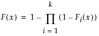
The mixture distribution's probability function F(x) is defined as follows:

where  is one of the supported distributions, k is the number of components in the mixture, and the wi are positive weights that sum to 1. The Fit Mixture option attempts to identify clusters of observations that are drawn from each of the component distributions, Fi(x). It estimates the parameters of the mixture and the probability that an observation is drawn from any given component.
Model Fit and Mixture Starting Value Methods
The fitting methodology is based on assumptions about the underlying clusters, called the Starting Value Method. Suppose that you designate k distributions. There are three Starting Value Methods:
• Single Cluster assumes that all observations are affected by all of the ingredient distributions to some extent. None of the densities stand out as affecting only a portion of the observations.
• Separable Clusters assumes that the ingredient distributions affect some observations more profoundly than others. For separable clusters, each of the k densities has an identifiable mode and defines a cluster.
• Overlapping Clusters assumes a situation that is intermediate between Single Cluster and Separable Clusters. Some densities stand out, but others jointly affect a portion of the observations. In this case, there are m clusters in the data, where m is less than k, the total number of densities.
The fitting process consists of these steps:
1. Clusters of observations are defined.
2. Assignment of clusters to densities is based on the Starting Value Method:
‒ For Separable Clusters, the highest likelihood assignment of clusters to the specified ingredient densities is determined by examining the possible permutations.
‒ For Overlapping Clusters, the highest likelihood assignment of clusters to the specified ingredient densities is determined by examining the possible permutations of clusters and combinations of observations.
Note: Suppose that you fit a model using a given Starting Value Method and then select another Starting Value Method. If a better fit based on the likelihood value cannot be achieved, no new model is added.
Mixture Control Panel
The control panel consists of these items:
Ingredient
Lists distributions that you can use as components of the fitted mixture distribution.
Quantity
Select the number of components in the mixture distribution that have the given distribution. The sum of the Quantity values is k, the number of densities in the mixture.
Starting Value Methods
Select a method that reflects your assumptions about the mixture. See “Model Fit and Mixture Starting Value Methods”.
Overlay
Shows the nonparametric estimates (Kaplan-Meier-Turnbull) for the uncensored data values. When you fit a mixture, the plot is updated to show the model and 95% level confidence bands. The confidence bands are not affected by the selection of Change Confidence Level in the Life Distribution red triangle menu. A Legend appears to the right of the plot.
Go
Click Go to fit the desired mixture. The Model List is updated with the model that you fit, and a report with the name of the mixture model is added.
Fit Mixture Reports
Model List
The Model List report lists the mixture distributions that you fit. The report provides the number of parameters, the number of actual observations, and the AICc, -2*LogLikelihood, and BIC statistics for each mixture distribution. For more details about these statistics, see the Statistical Details appendix in the Fitting Linear Models book.
Note the following:
• Smaller values of each of these statistics indicate a better fit.
• The rows are sorted by AICc.
• The Comparison Criterion red triangle option does not affect the order of models in the Model List.
• The AICc, -2*LogLikelihood, and BIC statistics also appear in the Model Comparisons table. This enables you to compare mixture distribution to other distributions for your data. See “Model Comparisons”.
Mixture Reports
The Model List report is followed by reports for each of the mixture distributions that you have fit. The title of each report describes the corresponding mixture using the specified ingredients and their quantities. The report lists the parameters, their estimates, standard errors, and 95% Wald confidence intervals. These intervals are not affected by the selection of Likelihood as the Confidence Interval Method in the launch window.
Parameter estimates are given for each distribution in the mixture. The Parameter column also includes parameters called Portion <i>, where i = 1, 2, .., k-1. These are estimates of the weights wi for the mixture. Since the weights sum to 1, the kth weight can be computed from the first k - 1 weights.
Density Overlay Plot
The Density Overlay plot shows estimates of the density functions for each of the components in the mixture. A legend to the right of the plot enables you to select which density functions appear.
Mixture Report Options
The red triangle menu contains the following options:
Remove
Removes the model report and the entry for the model in the Model List.
Show Profilers
Shows four types of profilers for the combined mixture distribution F. See “Mixture Profiler Options” for a description of their red triangle options.
‒ The Distribution Profiler shows cumulative failure probability as a function of time.
‒ The Quantile Profiler shows failure time as a function of cumulative probability.
‒ The Hazard Profiler shows the hazard rate as a function of time.
‒ The Density Profiler shows the density function for the distribution.
Save Predictions
For each mixture density, saves a column to the data table containing the probability that an observation belongs to that density. For the formulas used in the calculation, see “Fit Mixture Save Predictions Formulas”.
Mixture Profiler Options
The profilers for each mixture report contain the following red triangle options:
Confidence Intervals
The Distribution, Quantile, and Hazard profilers show 95% Wald-based confidence curves for the plotted functions. This option shows or hides the confidence curves. The confidence level is not affected when you select Change Confidence Level from the Life Distribution red triangle menu.
Note: To reduce computation time, the confidence intervals provided in the profilers are based on the Wald method, even if the Likelihood Confidence Interval Method is selected in the launch window.
Reset Factor Grid
Displays a window for each factor allowing you to enter a specific value for the factor’s current setting, to lock that setting, and to control aspects of the grid. For details, see the Profiler chapter in the Profilers book.
Factor Settings
Provides a menu that consists of options relating to profiler settings, scripts, and linking profilers. For details, see the Profiler chapter in the Profilers book.
Example of Fit Mixture
In this example, you fit two mixture distributions and then identify observations belonging to one of the clusters for the second mixture.
Fitting Two Mixture Distributions
1. Select Help > Sample Data Library and open Reliability/Mixture Demo.jmp.
2. Select Analyze > Reliability and Survival > Life Distribution.
3. Select Y1 and click Y, Time to Event.
4. Click OK.
5. Select Fit Mixture from the red triangle menu next to Life Distribution.
6. Type 2 in the Quantity box next to Weibull.
7. Select Separable Clusters in the Starting Value Methods panel.
8. Click Go.
Figure 3.9 Fit Mixture for Weibull (2)

JMP fits a mixture model consisting of two Weibull components. Portion 1 is estimated as 0.231688, indicating that approximately 23% of observations have the Weibull distribution with alpha = 9.483152 and beta = 3.001962. The remaining 77% are estimated to come from the second Weibull distribution.
To compare this model to another, you can change the Ingredient selections and the Quantity of components.
9. Type 1 next to Lognormal and 1 next to Weibull.
10. Click Go.
Figure 3.10 Fit Mixture for Lognormal(1), Weibull(1)

The Overlay plot is updated to show both mixture models. The plots and statistics in the Model List indicate that the Lognormal(1), Weibull(1) mixture seems to give a fit that is very similar to the Weibull(2) mixture.
Identifying Observations Belonging to a Cluster
1. From the Lognormal(1), Weibull(1) red triangle menu, select Save Predictions.
Two columns are added to the data table:
‒ Lognormal(1), Weibull(1) - Predicted Probability from Lognormal
‒ Lognormal(1), Weibull(1) - Predicted Probability from Weibull
2. Select Analyze > Distribution.
3. Select the two new columns from the Select Columns list and click Y, Columns.
4. Check Histograms Only.
5. Click OK.
6. In the histogram for Lognormal(1), Weibull(1) - Predicted Probability from Weibull, click in the bar corresponding to the value near 1.
Figure 3.11 Histograms for Mixture Probabilities
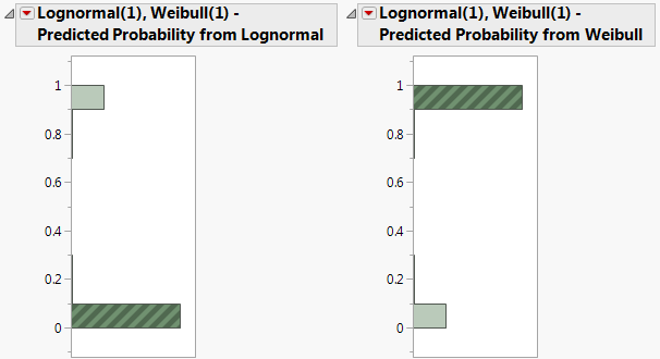
In the data table, the 297 corresponding rows are selected. These are the observations that are likely to have come from the Weibull distribution with parameters alpha = 29.90 and beta = 10.41.
Fit Competing Risk Mixture
The Fit Competing Risk Mixture option enables you to fit competing risk mixture distributions. It estimates the probability that a given observation fails due to the cause represented by each of the component mixture distributions.
The competing risk mixture probability distribution function F(x) is defined as follows:
where  represents the cumulative failure distributions for the ith risk and k is the number of components (or risks) in the mixture. The Fit Competing Risk Mixture option attempts to identify clusters of observations that are drawn from each of the component distributions, Fi(x). It estimates the parameters of the mixture and the probability that an observation is drawn from any given component.
The Competing Risk Mixture report is structured in a fashion that mirrors the Mixture report. See “Mixture”. However, the Fit Competing Risk Mixture reports do not show a Density Overlay plot. They show a Distribution Overlay plot instead.
Distribution Overlay Plot
The Distribution Overlay plot shows the cumulative distribution functions for each of the mixture components and for the combined mixture (Aggregated). A legend to the right of the plot enables you to select which cumulative distribution functions appear.
Weibayes Report
If you have data with zero failures (right-centered) and you have not turned off the preference Weibayes Only for Zero Failure Data, a special Weibayes report appears. Figure 3.12 shows the Weibayes report for the Weibayes No Failures.jmp sample data table, found in the Reliability folder.
Figure 3.12 Weibayes Report
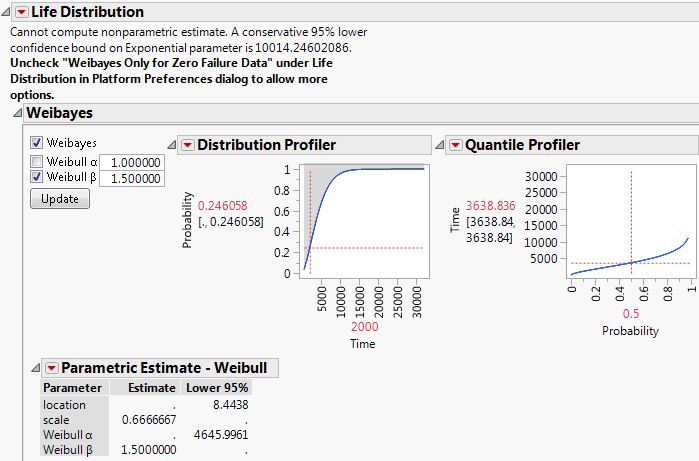
The analysis begins by assuming an exponential model. The note at the top of the report provides a lower confidence bound for the parameter of an exponential distribution. This lower confidence bound is computed using the method described in Section 7.7, page 167, of Meeker (1998).
The Weibayes section of the report conducts the Weibayes analysis. For a description of the procedure, see Nelson (1985).
To obtain Weibayes estimates, make sure that Weibayes and Weibull β options are selected. Change the Weibull β value and click Update. The estimates and profilers are updated. The values shown in the profilers use the conservative confidence bound. For an example, see “Weibayes Example for Data with No Failures”.
Note: If you deselect the Weibayes option, JMP shows the fixed parameter MLE.
When your data table contains at least one failure, a full Life Distribution report appears, but the maximum likelihood inference might not produce useful results. In this instance, a Weibayes analysis might be preferable. For an example, see “Weibayes Example for Data with One Failure”.
Note: To conduct Bayesian inference using the usual Life Distribution options when you have zero-failure data, deselect the Weibayes Only for Zero Failure Data preference and relaunch the analysis.
Competing Cause Report
Tip: If you find that the report window is too long, select Tabbed Report from the red triangle menu.
The Competing Cause report appears if you have assigned a Failure Cause column in the launch window. Use this report to analyze the competing causes to determine which causes are influential. For an example of this report, see “Omit Competing Causes”. For technical details, see “Competing Cause Details”.
The Competing Cause report contains the following content and options:
Competing Cause Workflow
Follow these steps to facilitate your use of the Competing Cause report:
1. For convenience, select the Tabbed Report option from the Competing Cause red triangle menu.
2. Select the Individual Causes tab. For each failure cause, use the options in its individual Life Distribution outline to select a distributional fit. See “Individual Causes”.
3. Select the Cause Combination tab. For each failure cause, specify the desired distribution in each Distribution list. See “Cause Combination”.
4. Click Update Model.
5. Select the Statistics tab to explore and save results for the model. See “Competing Cause: Statistics”.
Note: Customizations made to the competing cause model report in the Statistics outline might be lost if you change the model and click Update Model again.
Competing Cause Model
In a competing cause situation, the aggregated failure function can be written as follows:

where Fi(x) is the cumulative failure distribution for the ith cause and k is the total number of causes. The function Fi(x) is cause-specific. It reflects the probability of failure due to cause i alone and does not account for other causes of failure.
An alternative formulation is given as follows:

where each  is a monotone increasing function with values in the interval [0, 1]. The function
  is called a subdistribution. This form of the aggregated failure distribution is used to predict proportions of failures that are associated with individual causes, accounting for failure due to other causes.
Cause Combination
The Cause Combination report lets you fit and compare different failure time distributions (Fi(x)) for the various causes. Different distributions are available based on selections that you have made in the launch window. Negative and zero-failure times are not allowed.
The default plot is based on a Linear scale and shows the following:
• Nonparametric estimates (Kaplan-Meier-Turnbull) for the uncensored data values and their confidence intervals. The confidence intervals are represented by horizontal blue lines.
• Fits of cumulative failure distributions (Fi(x)) to each of the causes. The initial distribution is the one that you selected in the launch window. If you selected Individual Best, the best distribution is computed for each group and these fits are shown. (This selection can be time-intensive.) If you selected Manual Pick, the initial Distribution is Nonparametric for all groups and nonparametric fits are shown. A legend appears to the right of the plot.
• The Aggregated cumulative failure distribution, F(x), represented by a black line. This function is computed based on the selected cause distribution. If a nonparametric distribution is specified for a cause, the aggregated cumulative failure distribution extends only as far as the final time observation for that cause.
As you interact with the report, statistics for the aggregated model are re-evaluated.
The Cause Combination report contains these elements:
Scale
Select the probability scale for the plot’s vertical axis. If a distribution fits well, then the points should follow a straight line when plotted on that scale. “Change the Scale” illustrates how changing the scale affects the distribution fit.
Omit
Check a box to remove the fit for the corresponding cause. Use this when a particular cause has been fixed. The Aggregated model updates to reflect the removal of the failures due to that cause. “Omit Competing Causes” illustrates the effect of omitting causes.
Cause
Lists the causes in the Cause column.
Distribution
Lists the available distributions for each cause. To change the distribution for a specific failure cause, select the distribution from the Distribution list. Click Update Model to show the new distribution fit on the plot. The Cause Summary report is also updated.
Count
Gives the number of observations with the given failure cause.
Update Model
Shows the selected distributions in the plot; updates the Cause Summary report with the selected models; adds the selected model as the most recent one in the Individual Causes report.
Competing Cause: Statistics
The Statistics report for Competing Cause contains the following reports:
Cause Summary Report
The Cause Summary report shows information for the fit defined by the current selections under Distribution in the Cause Summary report. The report shows the number of failures for each cause and the parameter estimates for the distribution fit to each failure cause. When you change distribution fits in the Cause Combination report and click Update Model, the Cause Summary report is updated.
The following information is provided:
• The Cause column shows either labels of causes or the censor code.
• The Counts column lists the number of failures for each cause.
• A numerical entry in the Counts column indicates that the cause has enough failure events to consider. A cause with fewer than two events is considered right censored. The column also identifies missing causes.
• The Distribution column specifies the selected distribution for each cause.
• Depending on the selected distributions, various columns display the parameters of the distributions:
‒ The location column specifies location parameters for various distributions.
‒ The scale column specifies scale parameters for various distributions. The Weibull α and Weibull β columns show Weibull estimates of alpha and beta.
‒ Other columns show parameters of other selected distributions.
‒ A Convergence column appears if there are convergence issues.
The Cause Summary red triangle menu options enable you to save the probability, quantile, hazard, and density estimates for the aggregated failure distribution to the data table.
Profilers
The Distribution, Quantile, Hazard, and Density profilers help you visualize the aggregated failure distribution. The Distribution, Quantile, and Hazard profilers show 95% level confidence bands. For further details, see “Profilers”.
Note: If a nonparametric distribution is specified for a cause, the Hazard and Density profilers are not provided. Also, confidence limits are not provided in the Distribution and Quantile profilers.
Individual Causes
The Individual Causes report contains Life Distribution - Failure Cause: <Distribution Name> reports for each of the individual causes. Each Life Distribution - Failure Cause: <Distribution Name> report shows plots and distributional fit statistics for the individual failure cause indicated in the report title.
Whenever you click Update Model in the Cause Combination report, any new cause distribution that you select is added to the Life Distribution - Failure Cause: <Distribution Name> report for that cause. In the Life Distribution - Failure Cause <Distribution Name> report, the following occur:
• The distribution is selected in the Compare Distributions report.
• The distribution is added to the Model Comparisons report.
• A Parametric report is added for that distribution.
Each Life Distribution - Failure Cause <Distribution Name> report is a Life Distribution: Statistics report as described in “Life Distribution: Statistics”. However, all confidence intervals are Wald intervals. These intervals are not affected by the selection of Likelihood as the Confidence Interval Method in the launch window.
Available Distributions for Competing Cause Compare Distributions Reports
If you specify a Failure Cause in the launch window, you can specify which groupings of distributions and models that you want to allow in the resulting Compare Distributions reports for Individual Causes. You can select ZI (Zero-Inflated), TH (Threshold), and DS (Defective Subpopulation) distributions. You can also select fixed parameter and Bayesian models.
Note: If you have disallowed any distributions in Preferences, these do not appear. Also, rules that govern which distributions appear for Life Distribution apply. See “Available Parametric Distributions”.
Competing Cause Report Options
The red triangle menu next to Competing Cause contains the following options:
Tabbed Report
Shows graphs and data on individual tabs rather than in the default outline style.
Tabbed Report for Individual Causes
Shows the Life Distribution - Failure Cause: <Distribution Name> reports in tabs, rather than as a stack of Life Distribution reports.
Show Points
Shows or hides data points in the Cause Combination plot. The Life Distribution platform uses the midpoint estimates of the step function to construct probability plots. When you deselect Show Points, the midpoint estimates are replaced by Kaplan-Meier estimates.
Show Subdistributions
Shows the profiler for each individual cause subdistribution  . See “Individual Subdistribution Profiler for Cause”.
Show Remaining Life Distribution
Shows the remaining life distribution through the Distribution Profiler. This is conditional upon the unit surviving through a given time.
Mean Remaining Life
Estimates the mean remaining life of a unit, given a survival time. In the Mean Remaining Life Calculator, enter a time value and press Enter to see the estimate and confidence limits. Click the plus sign to enter additional times. Click the minus sign to remove the most recent entry.
To obtain a confidence interval, select the Configuration option from the Mean Remaining Life Calculator. Check Use bootstrap to construct confidence intervals. Enter appropriate values, keeping in mind that computation can be time-intensive. For details, see “Mean Remaining Life Calculator”.
Export Bootstrap Results
Appears only when a Bayesian model is selected and when Update Model has been applied.
Bootstrap Sample Size
When Bayesian Estimates or Weibayes results are used for any cause, the confidence limits for aggregated functions that appear in the Distribution Profiler must be simulated using parametric bootstrap. Use this option to specify the number of samples to be used in the bootstrap. See “Specify a Bayesian Model for a Cause”.
See the JMP Reports chapter in the Using JMP book for more information about the following options:
Local Data Filter
Shows or hides the local data filter that enables you to filter the data used in a specific report.
Redo
Contains options that enable you to repeat or relaunch the analysis. In platforms that support the feature, the Automatic Recalc option immediately reflects the changes that you make to the data table in the corresponding report window.
Save Script
Contains options that enable you to save a script that reproduces the report to several destinations.
Save By-Group Script
Contains options that enable you to save a script that reproduces the platform report for all levels of a By variable to several destinations. Available only when a By variable is specified in the launch window.
Individual Subdistribution Profiler for Cause
For a given cause, the Individual Subdistribution Profiler for Cause shows the estimated probability of failure, , from that cause at time t. The estimated probability takes into account failures from competing causes. See “Competing Cause Model”.
To show a profiler of the subdistribution for each cause, select Show Subdistributions from the Competing Cause red triangle menu. The Individual Subdistribution Profiler for Cause report appears beneath the other profilers. It consists of a profiler and a calculator.
Note: When you select Show Subdistributions, the Cause Combination plot is updated to show the subdistribution functions for all causes.
Select a Cause from the list to the right of the profiler to see its profiler. Options that apply to the profiler are provided in the Individual Subdistribution Profiler for Cause red triangle menu. See “Profilers”.
Use the Calculator panel to find values of the subdistribution functions for all causes at one or more Time to Event values. Enter a value for the Time to Event variable. When you press Enter (or click outside the text box), values for each of the causes are updated. To add a Time to Event value, click the plus sign. To remove the most recent value, click the minus sign.
Life Distribution - Compare Groups Report
Tip: If you find that the report window is getting too long, select Tabbed Report from the red triangle menu.
If you selected the Compare Groups tab in the launch window, the Life Distribution - Compare Groups report appears. This report compares different groups using a single specified distribution. For example, you might compare Weibull fits for components grouped by supplier. In contrast, the Life Distribution tab compares several fitted distributions for a single group.
You can compare the CDF, Quantile, Hazard, and Density functions. You can also consolidate the probability and quantile predictions of all groups.
For an example of this report, see “Examine the Same Distribution across Groups”.
The Compare Groups report can contain the following content and options:
• “Compare Distributions” (no Distribution Profiler)
Compare Groups: Statistics
The Statistics report for Compare Groups contains the following reports:
Summary
The Summary report contains a row for each group and for the combined data. Each row shows the number of units that failed and the numbers that were left, interval, or right censored. Each row also gives the corresponding mean and standard error. For details about how the mean and standard error are computed, see “Statistical Reports for Survival Analysis” in the “Survival Analysis” chapter.
Wilcoxon Group Homogeneity Test
This report presents results of the Wilcoxon test for equality of the failure functions. The report gives the chi-square approximation, the associated degrees of freedom, and the p-value for the test. A small p-value suggests that the groups differ. For an example, see “Wilcoxon Group Homogeneity Test” in the “Fit Life by X” chapter. The Wilcoxon test and its generalization to censored data are discussed in Kalbfleisch and Prentice (1980).
Parameter Estimates
The Parameter Estimates outline contains reports entitled Parametric Estimate - <Distribution Name> for each distribution that is fit. For each group, the Parametric Estimate - <Distribution Name> report gives the distribution’s parameter estimates and their 95% level confidence intervals. The confidence level is not affected when you select Change Confidence Level from the Life Distribution - Compare Groups red triangle menu.
Individual Group
The tabs within the Individual Group report contain Life Distribution reports for each individual group. For details about these reports, see “Life Distribution Report” and “Life Distribution Report Options”.
Life Distribution - Compare Groups Report Options
Many of the options in the Compare Groups red triangle menu can also be found in the Life Distribution red triangle menu. See “Life Distribution Report Options”.
However, the following options are specific to Compare Groups:
Show Quantile Functions
Shows or hides the Compare Quantile report. Select a distribution. For each group, a curve is plotted showing the estimated quantiles for the time variable. Confidence bands are displayed. A legend is shown to the right of the plot. Only one distribution can be specified at a time.
Show Hazard Functions
Shows or hides the Compare Hazard report. Select a distribution. For each group, a curve is plotted showing the hazard function. Confidence bands are displayed. A legend is shown to the right of the plot. Only one distribution can be specified at a time.
Show Density Functions
Shows or hides the Compare Density report. Select a distribution. For each group, the density function and confidence bands are displayed. A legend is shown to the right of the plot. Only one distribution can be specified at a time.
Estimate Probability
Adds an Estimate Probability report corresponding to the most recently selected distribution under Compare Distribution. Enter a value for the Time to Event variable in the text box and press Enter. To add a Time to Event value, click the plus sign. To remove the most recent value, click the minus sign. For further details, see “Estimate Probability Report”.
Estimate Quantile
(Appears only if Compare Quantile is selected.) Adds an Estimate Quantile report corresponding to the most recently selected distribution under Compare Quantile. Enter a value for the probability of interest in the text box and press Enter. To add a Prob value, click the plus sign. To remove the most recent value, click the minus sign. For each group and probability value, the Time to Event quantile and 95% Wald and Likelihood confidence intervals are shown.
Estimate Probability Report
For each group and Time to Event value, this report provides the following:
Midpoint Estimate
Midpoint-adjusted Kaplan-Meier estimate of failure by the specified time.
Lower 95%, Upper 95%
Pointwise 95% confidence intervals for the probability of failure by the specified time.
Simultaneous Lower 95% (Nair), Simultaneous Upper 95% (Nair)
Simultaneous 95% confidence intervals for the probability of failure by the specified time. See Nair (1984) and Meeker and Escobar (1998).
Survival Probability
Midpoint-adjusted estimate of survival beyond the specified time.
Survival Probability Lower 95%, Upper 95%
Pointwise 95% confidence intervals for the probability of survival beyond the specified time.
Survival Probability Simultaneous Lower 95% (Nair), Simultaneous Upper 95% (Nair)
Simultaneous 95% confidence intervals for the probability of survival beyond the specified time. See Nair (1984) and Meeker and Escobar (1998).
Additional Examples of the Life Distribution Platform
This section includes examples of omitting competing causes and changing the distribution scale.
Omit Competing Causes
This example illustrates how to decide on the best fit for competing causes.
1. Select Help > Sample Data Library and open Reliability/Blenders.jmp.
2. Select Analyze > Reliability and Survival > Life Distribution.
3. Select Time Cycles and click Y, Time to Event.
4. Select Causes and click Failure Cause.
5. Select Censor and click Censor.
6. Select Individual Best as the Distribution.
7. Make sure that AICc is the Comparison Criterion.
8. Click OK.
On the Competing Cause report, JMP shows the best distribution fit for each failure cause.
Figure 3.13 Initial Competing Cause Report

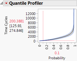
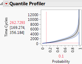
9. In the Quantile Profiler, type 0.1 for the probability.
The estimated time by which 10% of the failures occur is 200.
Figure 3.14 Estimated Failure Time for 10% of the Units
10. Select Omit for bearing seal, belt, container throw, cord short, and engine fan (the causes with the fewest failures).
The estimated time by which 10% of the failures occur is now 263.
Figure 3.15 Updated Failure Time
When power switch and stripped gear are the only causes of failure, the estimated time by which 10% of the failures occur increases by approximately 31%.
Change the Scale
In the initial Compare Distributions report, the probability and time axes are linear. But suppose that you want to see distribution estimates on a Fréchet scale.1
2. In the Compare Distributions report, select Fréchet in the Scale column.
3. Select Interval Type > Pointwise from the red triangle menu.
Figure 3.16 Nonparametric Estimates with a Fréchet Probability Scale
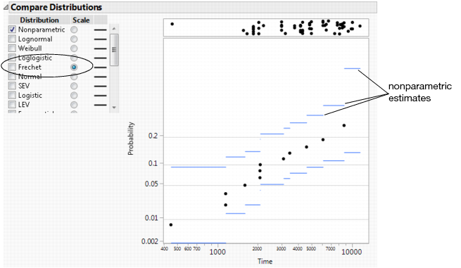
Using a Fréchet scale, the nonparametric estimates approximate a straight line, meaning that a Fréchet fit might be reasonable.
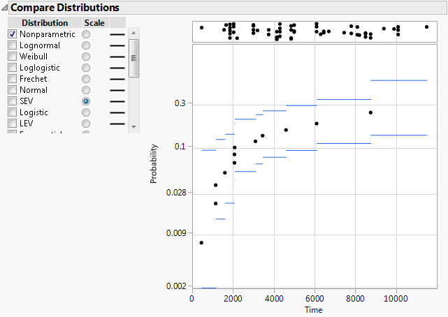
4. Select SEV in the Scale column.
The nonparametric estimates no longer approximate a straight line (Figure 3.17). You now know that the SEV distribution is not appropriate.
Figure 3.17 Nonparametric Estimates with a SEV Probability Scale
Examine the Same Distribution across Groups
Suppose you want to compare the same distribution across different groups. You want to examine estimates of failure probabilities for a single type of capacitor operating at three different temperatures.
1. Select Help > Sample Data Library and open Reliability/Capacitor ALT.jmp.
2. Select Analyze > Reliability and Survival > Life Distribution.
3. Click the Compare Groups tab.
4. Select Hours and click Y, Time to Event.
5. Select Temperature and click Grouping.
6. Select Censor and click Censor.
7. Select Freq and click Freq.
8. Click OK.
Figure 3.18 Compare Distribution for Groups
The default graph shows the nonparametric estimates. At a higher temperature, the capacitor has a higher probability of failure. You want to try fitting a parametric distribution.
9. Select Weibull for Distribution and Scale.
Figure 3.19 Compare Weibull Distribution for Groups

When plotted against a Weibull probability scale, the points come close to following three lines. This indicates that a Weibull distribution provides a reasonable fit for each of the Temperature groups.
Weibayes Estimates
There are two possible ways to obtain a Weibayes analysis:
• You have no failures (all observations are right-censored) and the preference Weibayes Only for Zero Failure Data is checked. Then the Weibayes report appears. See “Weibayes Example for Data with No Failures”.
• You have few failures. A full Life Distribution report is presented. Fit a Weibull distribution. In the Parametric Estimate - Weibull report, select the Fix Parameter option. Then select the Weibayes option in the Fixed Parameter report. See “Weibayes Example for Data with One Failure”.
Weibayes Example for Data with No Failures
You have data for a product that is mostly reliable. Thirty were tested for 1,000 hours with no failures occurring. You want to predict the failure probability at 2,000 hours.
1. Select Help > Sample Data Library and open Reliability/Weibayes No Failures.jmp.
2. Select Analyze > Reliability and Survival > Life Distribution.
3. Select Time and click Y, Time to Event.
4. Select Censor and click Censor.
5. Select Freq and click Freq.
6. Select Likelihood as the Confidence Interval Method.
7. Click OK.
A special Life Distribution report appears. Weibayes and Weibull beta should be selected.
8. Type 1.5 as the known Weibull β value.
The value 1.5 is considered appropriate for this example.
9. Click Update.
10. In the Distribution Profiler, type 2000 for Time.
Figure 3.20 Life Distribution Report for Zero Failures
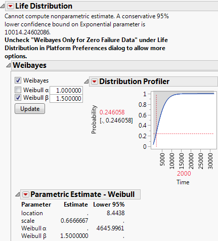
From the Distribution Profiler, you can see that at 2,000 hours, the conservative probability is 24.6058%. That means that the one-tailed lower 95% confidence limit for the failure probability is 24.6058%.
Weibayes Example for Data with One Failure
Suppose you have the same data, but this time, one failure occurred at 800 hours. Again, you want to predict the failure probability at 2,000 hours.
1. Select Help > Sample Data Library and open Reliability/Weibayes One Failure.jmp.
2. Select Analyze > Reliability and Survival > Life Distribution.
3. Select Time and click Y, Time to Event.
4. Select Censor and click Censor.
5. Select Freq and click Freq.
6. Select Likelihood as the Confidence Interval Method.
7. Click OK.
The Life Distribution report appears.
8. Select the Weibull distribution in the Compare Distributions plot.
9. Select Fix Parameter from the Parametric Estimate - Weibull red triangle menu.
10. Select Weibayes and Weibull beta in the Fix Parameter report.
11. Type 1.5 as the known Weibull β value.
12. Click Update.
13. In the Distribution Profiler, type 2000 for Time.
14. Place your cursor over the top of the Y axis. The cursor becomes a hand. Drag the axis downward until it reaches 0.5 as the top number.
Figure 3.21 Life Distribution Report for One Failure
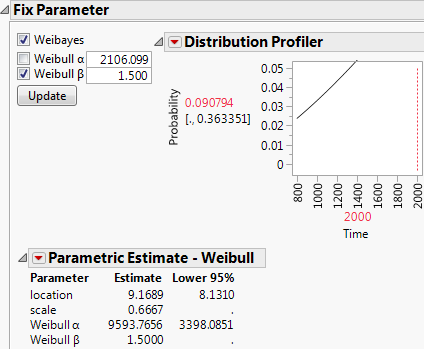
In the Distribution Profiler, the solid line shows the MLE. The dashed line shows the Weibayes conservative limit. You can see that at 2,000 hours, the conservative probability is 36.3351%. That means that the one-tailed lower 95% confidence limit for the failure probability is 36.3351%.
Technical Details
This section covers the following topics:
• The distributions used in the Life Distribution platform. See “Distributions”.
• Technical information about the Competing Cause report. See “Competing Cause Details”.
Distributions
This section provides details for the distributional fits in the Life Distribution platform. Meeker and Escobar (1998, Chapters 2-5) is an excellent source of theory, application, and discussion for both the nonparametric and parametric details that follow.
Estimation and Confidence Intervals
The parameters of all distributions, unless otherwise noted, are estimated using maximum likelihood estimates (MLEs). The only exceptions are the threshold distributions. If the smallest observation is an exact failure, then this observation is treated as interval-censored with a small interval. The parameter estimates are the MLEs estimated from this slightly modified data set. Without this modification, the likelihood can be unbounded, so an MLE might not exist. This approach is similar to that described in Meeker and Escobar (1998, p. 275), except that only the smallest exact failure is censored. This is the minimal change to the data that guarantees boundedness of the likelihood function.
The Life Distribution platform offers two methods for calculating confidence intervals for the distribution parameters. These methods are labeled as Wald or Likelihood and can be selected in the launch window for the Life Distribution platform. Wald confidence intervals are used as the default setting. The computations for the confidence intervals for the cumulative distribution function (cdf) start with Wald confidence intervals on the standardized variable. Next, the intervals are transformed to the cdf scale (Nelson, 1982, pp. 332-333 and pp. 346-347). The confidence intervals given in the other graphs and profilers are transformed Wald intervals (Meeker and Escobar, 1998, chap. 7). Joint confidence intervals for the parameters of a two-parameter distribution are shown in the log-likelihood contour plots. They are based on approximate likelihood ratios for the parameters (Meeker and Escobar, 1998, chap. 8).
Nonparametric Fit
A nonparametric fit describes the basic curve of a distribution. For data with no censoring (failures only) and for data where the observations consist of both failures and right-censoring, JMP uses Kaplan-Meier estimates. For mixed, interval, or left censoring, JMP uses Turnbull estimates. When your data set contains only right-censored data, the Nonparametric Estimate report indicates that the nonparametric estimate cannot be calculated.
The Life Distribution platform uses the midpoint estimates of the step function to construct probability plots. The midpoint estimate is halfway between (or the average of) the current and previous Kaplan-Meier estimates.
Parametric Distributions
Parametric distributions provide a more concise distribution fit than nonparametric distributions. The estimates of failure-time distributions are also smoother. Parametric models are also useful for extrapolation (in time) to the lower or upper tails of a distribution.
Note: Many distributions in the Life Distribution platform are parameterized by location and scale. For lognormal fits, the median is also provided. A threshold parameter is also included in threshold distributions. Location corresponds to μ, scale corresponds to σ, and threshold corresponds to γ.
Lognormal
Lognormal distributions are used commonly for failure times when the range of the data is several powers of 10. This distribution is often considered as the multiplicative product of many small positive identically independently distributed random variables. It is reasonable when the log of the data values appears normally distributed. Examples of data appropriately modeled by the lognormal distribution include hospital cost data, metal fatigue crack growth, and the survival time of bacteria subjected to disinfectants. The pdf curve is usually characterized by strong right-skewness. The lognormal pdf and cdf are:

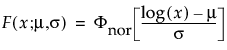 ,
,where
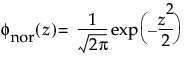
and
are the pdf and cdf, respectively, for the standardized normal, or nor(μ = 0, σ = 1) distribution.
Weibull
The Weibull distribution can be used to model failure time data with either an increasing or a decreasing hazard rate. It is used frequently in reliability analysis because of its tremendous flexibility in modeling many different types of data, based on the values of the shape parameter, β. This distribution has been successfully used for describing the failure of electronic components, roller bearings, capacitors, and ceramics. Various shapes of the Weibull distribution can be revealed by changing the scale parameter, α, and the shape parameter, β. The Weibull pdf and cdf are commonly represented as follows:
 ,
,where α is a scale parameter, and β is a shape parameter. The Weibull distribution is particularly versatile because it reduces to an exponential distribution when β = 1. An alternative parameterization commonly used in the literature and in JMP is to use σ as the scale parameter and μ as the location parameter. These are easily converted to an α and β parameterization by
and
The pdf and the cdf of the Weibull distribution are also expressed as a log-transformed smallest extreme value distribution (SEV). This uses a location scale parameterization, with μ = log(α) and σ = 1/β,
where
and
are the pdf and cdf, respectively, for the standardized smallest extreme value (μ = 0, σ = 1) distribution.
Loglogistic
The pdf of the loglogistic distribution is similar in shape to the lognormal distribution but has heavier tails. It is often used to model data exhibiting non-monotonic hazard functions, such as cancer mortality and financial wealth. The loglogistic pdf and cdf are:

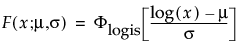 ,
,where

and
are the pdf and cdf, respectively, for the standardized logistic or logis distribution(μ = 0, σ = 1).
Fréchet
The Fréchet distribution is known as a log-largest extreme value distribution or sometimes as a Fréchet distribution of maxima when it is parameterized as the reciprocal of a Weibull distribution. This distribution is commonly used for financial data. The pdf and cdf are:
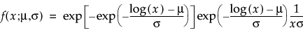

and are more generally parameterized as
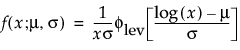

where
and
are the pdf and cdf, respectively, for the standardized largest extreme value LEV(μ = 0, σ = 1) distribution.
Normal
The normal distribution is the most widely used distribution in most areas of statistics because of its relative simplicity and the ease of applying the central limit theorem. However, it is rarely used in reliability. It is most useful for data where μ > 0 and the coefficient of variation (σ/μ) is small. Because the hazard function increases with no upper bound, it is particularly useful for data exhibiting wear-out failure. Examples include incandescent light bulbs, toaster heating elements, and mechanical strength of wires. The pdf and cdf are:
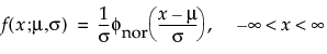

where

and

are the pdf and cdf, respectively, for the standardized normal, or nor(μ = 0, σ = 1) distribution.
Smallest Extreme Value (SEV)
This non-symmetric (left-skewed) distribution is useful in two cases. The first case is when the data indicate a small number of weak units in the lower tail of the distribution (the data indicate the smallest number of many observations). The second case is when σ is small relative to μ, because probabilities of being less than zero, when using the SEV distribution, are small. The smallest extreme value distribution is useful to describe data whose hazard rate becomes larger as the unit becomes older. Examples include human mortality of the aged and rainfall amounts during a drought. This distribution is sometimes referred to as a Gumbel distribution. The pdf and cdf are:


where
and
are the pdf and cdf, respectively, for the standardized smallest extreme value, SEV(μ = 0, σ = 1) distribution.
Logistic
The logistic distribution has a shape similar to the normal distribution, but with longer tails. The logistic distribution is often used to model life data when negative failure times are not an issue. Logistic regression models for a binary or ordinal response assume the logistic distribution as the latent distribution. The pdf and cdf are:

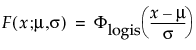
where
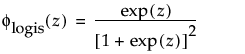
and
are the pdf and cdf, respectively, for the standardized logistic or logis distribution (μ = 0, σ = 1).
Largest Extreme Value (LEV)
This right-skewed distribution can be used to model failure times if σ is small relative to μ > 0. This distribution is not commonly used in reliability but is useful for estimating natural extreme phenomena, such as a catastrophic flood heights or extreme wind velocities. The pdf and cdf are:


where
and
are the pdf and cdf, respectively, for the standardized largest extreme value LEV(μ = 0, σ = 1) distribution.
Exponential
Both one- and two-parameter exponential distributions are used in reliability. The pdf and cdf for the two-parameter exponential distribution are:
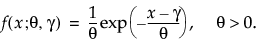

where θ is a scale parameter and γ is both the threshold and the location parameter. Reliability analysis frequently uses the one-parameter exponential distribution, with γ = 0. The exponential distribution is useful for describing failure times of components exhibiting wear-out far beyond their expected lifetimes. This distribution has a constant failure rate, which means that for small time increments, failure of a unit is independent of the unit’s age. The exponential distribution should not be used for describing the life of mechanical components that can be exposed to fatigue, corrosion, or short-term wear. This distribution is, however, appropriate for modeling certain types of robust electronic components. It has been used successfully to describe the life of insulating oils and dielectric fluids (Nelson, 1990, p. 53).
Log Generalized Gamma (LogGenGamma)
The log generalized gamma distribution contains the SEV, LEV, and Normal. The pdf and cdf are:
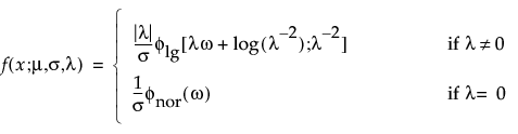
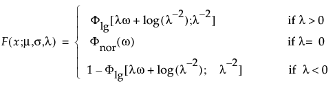
where  , ω = [x – μ]/σ, and
Note that
are the pdf and cdf, respectively, for the log-gamma variable and κ > 0 is a shape parameter. The standardized distributions above are dependent upon the shape parameter κ.
Note: In JMP, the shape parameter, λ, for the generalized gamma distribution is bounded between [-12,12] to provide numerical stability.
Extended Generalized Gamma (GenGamma)
The extended generalized gamma distribution can include many other distributions as special cases, such as the generalized gamma, Weibull, lognormal, Fréchet, gamma, and exponential. It is particularly useful for cases with little or no censoring. This distribution has been successfully modeled for human cancer prognosis. The pdf and cdf are:


where x > 0, ω = [log(x) – μ]/σ, and
Note that
are the pdf and cdf, respectively, for the standardized log-gamma variable and κ > 0 is a shape parameter.
The standardized distributions above are dependent upon the shape parameter κ. Meeker and Escobar (chap. 5) give a detailed explanation of the extended generalized gamma distribution.
Note: In JMP, the shape parameter, λ, for the generalized gamma distribution is bounded between [-12,12] to provide numerical stability.
Distributions with Threshold Parameters
Threshold Distributions are log-location-scale distributions with threshold parameters. Some of the distributions above are generalized by adding a threshold parameter, denoted by γ. The addition of this threshold parameter shifts the beginning of the distribution away from 0. Threshold parameters are sometimes called shift, minimum, or guarantee parameters because all units survive the threshold. Note that while adding a threshold parameter shifts the distribution on the time axis, the shape, and spread of the distribution are not affected. Threshold distributions are useful for fitting moderate to heavily shifted distributions. The general forms for the pdf and cdf of a log-location-scale threshold distribution are:

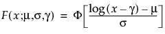
where φ and Φ are the pdf and cdf, respectively, for the specific distribution. Examples of specific threshold distributions are shown below for the Weibull, lognormal, Fréchet, and loglogistic distributions, where, respectively, the SEV, Normal, LEV, and logis pdfs and cdfs are appropriately substituted.
TH Weibull
The pdf and cdf of the three-parameter Weibull distribution are:

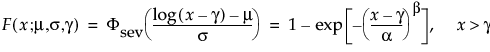
where μ =log(α), and σ= 1/β and where
and
are the pdf and cdf, respectively, for the standardized smallest extreme value, SEV(μ = 0, σ = 1) distribution.
TH Lognormal
The pdf and cdf of the three-parameter lognormal distribution are:


where

and
are the pdf and cdf, respectively, for the standardized normal, or N(μ = 0, σ = 1) distribution.
TH Fréchet
The pdf and cdf of the three-parameter Fréchet distribution are:
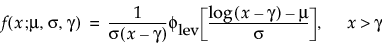
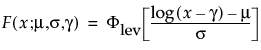
where
and
are the pdf and cdf, respectively, for the standardized largest extreme value LEV(μ = 0, σ = 1) distribution.
TH Loglogistic
The pdf and cdf of the three-parameter loglogistic distribution are:
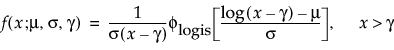

where

and
are the pdf and cdf, respectively, for the standardized logistic or logis distribution (μ = 0, σ = 1).
Distributions for Defective Subpopulations
In reliability experiments, there are times when only a fraction of the population has a particular defect leading to failure. Because all units are not susceptible to failure, using the regular failure distributions is inappropriate and might produce misleading results. Use the DS distribution options to model failures that occur on only a subpopulation. The following DS distributions are available:
• DS Lognormal
• DS Weibull
• DS Loglogistic
• DS Fréchet
Zero-Inflated Distributions
Zero-inflated distributions are used when some proportion (p) of the data fail at t = 0. When the data contain more zeros than expected by a standard model, the number of zeros is inflated. When the time-to-event data contain zero as the minimum value in the Life Distribution platform, four zero-inflated distributions are available. These distributions include:
• Zero-Inflated Lognormal (ZI Lognormal)
• Zero-Inflated Weibull (ZI Weibull)
• Zero-Inflated Loglogistic (ZI Loglogistic)
• Zero-Inflated Fréchet (ZI Fréchet)
The pdf and cdf for zero-inflated distributions are


where:
p is the proportion of zero data values,
t is the time of measurement for the lifetime event,
μ and σ are estimated by calculating the usual maximum likelihood estimations after removing zero values from the original data,
φ(z) and Φ(z) are the density and cumulative distribution function, respectively, for a standard distribution. For example, for a Weibull distribution,
φ(z) = exp(z-exp(z)) and Φ(z) = 1 - exp(-exp(z)).
See Lawless (2003, p 34) for a more detailed explanation of using zero-inflated distributions. Substitute p = 1 - p and S1(t) = 1 - Φ(t) to obtain the form shown above.
See Tobias and Trindade (1995, p 232) for additional information about reliability distributions. This reference gives the general form for mixture distributions. Using the parameterization in Tobias and Trindade, the form above can be found by substituting α = p, Fd(t) = 1, and FN(t) = Φ(t).
Prior Distributions for Bayesian Estimation
The following distributions are available for Location Scale Priors:
• Normal/Lognormal, with hyperparameters Location (mu) and Scale (sigma). For a definition, see “Lognormal” and “Normal”.
• Uniform, with hyperparameters Low and End, which define the support of a Uniform distribution.
• Gamma, with hyperparameters Shape and Scale. The k/theta parameterization and the probability density function is used.
• Point Mass, with hyperparameter Location. This is a degenerated prior; there is only one possible value for the parameter that we are assigning a prior distribution to. The only possible value equals the value that is entered to this Location hyperparameter.
The following distributions are available for Quantile Parameter Priors:
• Normal/Lognormal, with a 99% probability range, specifies the prior distribution using the 0.005 and 0.995 percentiles of the distribution. JMP backs out the mu and sigma.
• Uniform, with hyperparameters Lower and Upper Limits, which define the support of a Uniform distribution.
• Log-Uniform, with Lower (a) and Upper (b) Limits, which are a distribution that is uniform on the log scale between Log(a) and Log(b).
• Point Mass, with hyperparameter Location. This is a degenerated prior; there is only one possible value for the parameter that we are assigning a prior distribution to. The only possible value equals the value that is entered to this Location hyperparameter.
The following distributions are available for Failure Probability Priors:
• Beta, characterized by the probability density function.
‒ Specify the Beta prior using estimates and error percentages (mean and variance). The mean equals the number entered in to the Estimate, and the variance equals (Error Percentage / 100 * Estimate)^2.
‒ Specify the Beta prior using 0.005 and 0.995 percentiles of the distribution. JMP backs out the hyperparameters.
Competing Cause Details
For a competing cause model, a closed form for the aggregated distribution is given as follows:
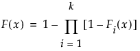
where the  , are individual failure distributions corresponding to causes. Confidence limits are readily available, because all involved estimates are MLEs.
Specify a Fixed Parameter Model as a Distribution for a Cause
If a Fixed Parameter model is specified for a cause, you must fix the parameter in the Individual Causes report for that cause. Fix the parameter in the desired Parametric Estimate report in the Life Distribution - Failure Cause: <Name> report. The fixed parameter becomes part of the aggregated distribution when you click Update Model.
The following example illustrates how to include the Fixed Parameter model into the aggregated distribution:
1. Select Help > Sample Data Library and open Reliability/Appliance.jmp.
2. Select Analyze > Reliability and Survival > Life Distribution.
3. Select Time Cycles and click Y, Time to Event.
4. Select Cause Code and click Failure Cause.
5. Select Likelihood as the Confidence Interval Method.
6. Select Allow failure mode to use fixed parameter models.
7. Click OK.
Figure 3.22 Fixed Parameter Model with Cause 1 Omitted

By default, Cause = 1 is omitted, because there are not enough data. However, you do not want this cause to be omitted.
8. Open the Individual Causes report for Cause 1. The report is called Life Distribution - Failure Cause: 1 Failure Counts: 1.
9. Select Fix Parameter from the red triangle next to Parametric Estimate - Weibull.
10. Select Weibull beta and type 2.
11. Click Update.
Figure 3.23 Fixed Parameter Model with Weibull Beta Specified
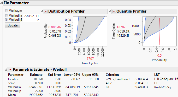
In the Parametric Estimate - Weibull report, assuming β equals 2, the alpha parameter is estimated to be 22463.391. Now you can use this for the failure distribution for Cause=1.
12. Scroll up to Cause Combination at the top of the report window.
13. Deselect Omit for Cause 1.
14. For the distribution for Cause 1, select Fixed Parameter Weibull.
15. Click Update Model.
Figure 3.24 Updated Model Showing Cause 1
Now the aggregated model uses the Fixed Parameter Weibull results for Cause 1 in the overall competing cause model.
Specify a Bayesian Model for a Cause
The steps for specifying a Bayesian model for a cause are similar to those described in “Specify a Fixed Parameter Model as a Distribution for a Cause”. Define the model in the desired Bayesian Estimation report found in the corresponding Parametric Estimate outline under Statistics in the Life Distribution report for the individual cause. See “Bayesian Estimation - <Distribution Name>”.
To incorporate a Bayesian model into the aggregated model, non-Bayesian distributions for other causes must be amenable to a simulation-based framework. For example, suppose that a model has two failure causes. One is modeled using a Weibull distribution and the other using a Bayesian approach for estimating the parameters of a second Weibull. The parameters for the first Weibull distribution, denoted by the vector θ1, are estimated using maximum likelihood. The parameters for the second Weibull, θ2, are estimated using the Bayesian approach.
The quantiles and median of the aggregated mixture distribution, denoted  , are obtained as follows:
• A parametric bootstrap is performed for the first Weibull, yielding random samples from the asymptotic distribution of the maximum likelihood estimate  . Denote a sampled value from the asymptotic distribution of
  by
by  .
.
• A sample is drawn from the posterior distribution of θ2, denoted by  .
.
• For each set of values  and
and  , an estimate of
  , denoted by
  , is obtained.
• The values  are used to obtain estimates of the quantiles and median of the aggregated distribution. These are the values displayed in the Distribution profiler at a given value of x.
Specify a Weibayes Model for a Cause
The steps for specifying a Weibayes model for a cause are similar to those described in “Specify a Fixed Parameter Model as a Distribution for a Cause”. Select the Fix Parameter option in the Parametric Estimate - Weibull outline under Statistics in the Life Distribution report for the cause. In the Fix Parameter report, check the Weibayes option. The Weibayes model is treated as a Bayesian model and a bootstrap sample is drawn from the posterior distribution of the parameter alpha. See Liu and Wang (2013).
Mean Remaining Life Calculator
Use the Configuration option in the red triangle menu to set a value for the number of simulated failure times used in computing the mean remaining life. Denote this value by m.
To obtain an estimate of the mean remaining life at time t, m samples are drawn from the aggregated distribution conditioned on survival to time t. Their average is computed.
To compute the confidence limits for the mean remaining life, you must select the box in the Configuration window. You then have the option to set the number of bootstrap samples. Denote this value by n.
To compute the confidence interval, n samples of parameter estimates are drawn from either the asymptotic distributions of the MLEs, or the posterior distributions derived using Bayesian inference. For each sample of parameter values, an aggregated distribution is formed, from which m samples are drawn to compute a mean remaining life. The samples of n mean remaining life values are used to construct the confidence interval.
Fit Mixture Save Predictions Formulas
This section gives the formulas used in calculating values in the columns saved by the Fit Mixture report option Save Predictions.
Consider the following notation:
‒ If the observation y is not censored, the saved value is given by
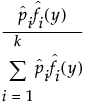
‒ If the observation is censored, the saved value is obtained by replacing the estimated density values in the formula for an uncensored observation by the following:
1 Using different scales is sometimes referred to as drawing the distribution on different types of probability paper.
..................Content has been hidden....................
You can't read the all page of ebook, please click here login for view all page.