
Fit Life by X Platform Overview
The Fit Life by X platform provides the tools needed for accelerated life-testing analysis. Accelerated tests are routinely used in industry to provide failure-time information about products or components in a relatively short time frame. Common accelerating factors include temperature, voltage, pressure, and usage rate. Results are extrapolated to obtain time-to-failure estimates at lower, normal operating levels of the accelerating factors. These results are used to assess reliability, detect and correct failure modes, compare manufacturers, and certify components.
The Fit Life by X platform includes many commonly used transformations to model physical and chemical relationships between the event and the factor of interest. Examples include transformation using Arrhenius (Celsius, Fahrenheit, and Kelvin) relationship time-acceleration factors and Voltage-acceleration mechanisms. Linear, Log, Logit, Reciprocal, Square Root, Box-Cox, Location, Location and Scale, and Custom acceleration models are also included in this platform.
You can use the DOE > Accelerated Life Test Design platform to design accelerated life test experiments. For more information, see the Design of Experiments Guide.
Meeker and Escobar (1998, p. 495) offer the following strategy for analyzing accelerated lifetime data:
1. Examine the data graphically. One useful way to visualize the data is by examining a scatterplot of the time-to-failure variable versus the accelerating factor.
2. Fit distributions individually to the data at different levels of the accelerating factor. Repeat for different assumed distributions.
3. Fit an overall model with a plausible relationship between the time-to-failure variable and the accelerating factor.
4. Compare the model in Step 3 with the individual analyses in Step 2, assessing the lack of fit for the overall model.
5. Perform residual and various diagnostic analyses to verify model assumptions.
6. Assess the plausibility of the data to make inferences.
Example of the Fit Life by X Platform
This example uses the Devalt.jmp sample data table, from Meeker and Escobar (1998), and can be found in the Reliability folder of the sample data. It contains time-to-failure data for a device at accelerated operating temperatures. No time-to-failure observation is recorded for the normal operating temperature of 10 degrees Celsius; all other observations are shown as time-to-failure or censored values at accelerated temperature levels of 40, 60, and 80 degrees Celsius.
1. Select Help > Sample Data Library and open Reliability/Devalt.jmp.
2. Select Analyze > Reliability and Survival > Fit Life by X.
3. Select Hours and clickY, Time to Event.
4. Select Temp and click X.
5. Select Censor and click Censor.
6. Leave the Censor Code as 1.
7. Select Weight and click Freq.
8. Keep Arrhenius Celsius as the relationship, and keep the Nested Model Tests option selected.
9. Select Weibull as the distribution.
10. Keep Wald as the confidence interval method.
Figure 4.2 shows the completed launch window.
Figure 4.2 Fit Life by X Launch Window
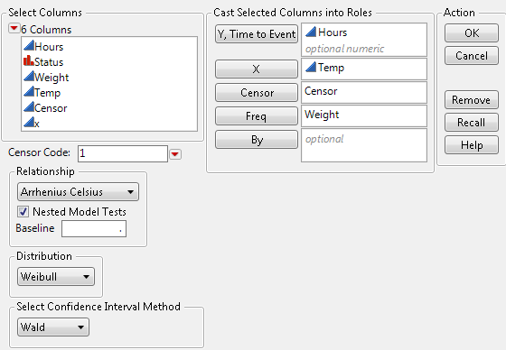
11. Click OK.
Figure 4.3 shows the top half of the Fit Life by X report window.
Note: A message might appear stating that “Analysis must exclude groups that are all right censored to continue Nested Model Tests. Do you want to continue?” Click Yes to continue the analysis. Right censored groups indicate groups where all observations are right censored. In this example, group Temp = 10 has only one row, is considered to be right censored, and has to be excluded to allow the Nested Model Test. The message does not appear if your sample data does not include right censored observations.
Figure 4.3 Fit Life by X Report Window for Devalt.jmp Data

The report window shows summary data, diagnostic plots, comparison data and results, including detailed statistics and prediction profilers. Separate result sections are shown for each selected distribution. Distribution, Quantile, Hazard, Density, and Acceleration Factor Profilers are included for each of the specified distributions.
Launch the Fit Life by X Platform
Launch the Fit Life by X platform by selecting Analyze > Reliability and Survival > Fit Life by X.
Figure 4.4 The Fit Life by X Launch Window
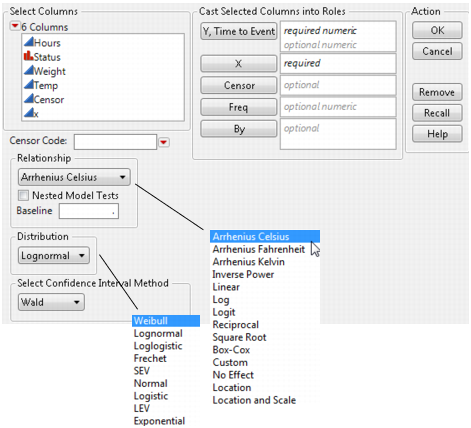
The Fit Life by X launch window contains the following options:
Y, Time to Event
Identifies the time to event (such as the time to failure) or time to censoring. With interval censoring, specify two Y variables, where one Y variable gives the lower limit and the other Y variable gives the upper limit for each unit. For details about censoring, see “Event Plot” in the “Life Distribution” chapter.
X
Identifies the accelerating factor.
Censor
Identifies censored observations. Select the value that identifies right-censored observations from the Censor Code menu beneath the Select Columns list. The Censor column is used only when one Y is entered.
Freq
Identifies frequencies or observation counts when there are multiple units. If the value is 0 or a positive integer, then the value represents the frequencies or counts of observations for each row when there are multiple units recorded.
By
Identifies a column that creates a report consisting of separate analyses for each level of the variable.
Censor Code
After selecting the Censor column, select the value that designates right-censored observations from the list. Missing values are excluded from the analysis. JMP attempts to detect the censor code and display it in the list.
Relationship
Determines the relationships between the event and the accelerating factor. Examples include transformation using the following acceleration models:
‒ Arrhenius Celsius: μ = b0 + b1 * 11605 / (X+273.15)
‒ Arrhenius Fahrenheit: μ = b0 + b1 * 11605 / ((X + 459.67)/1.8)
‒ Arrhenius Kelvin: μ = b0 + b1 * 11605/X
‒ Voltage: μ = b0 + b1 * log (X)
‒ Linear: μ=b0 + b1* X
‒ Log: μ = b0 + b1 * log(X)
‒ Logit: μ = b0 + b1 * log(X/(1-X))
‒ Reciprocal: μ = b0 + b1/X
‒ Square Root: μ = b0 + b1 * sqrt(X)
‒ Box-Cox: μ = b0 + b1 * Boxcox(X)
‒ Location: means μ is different for every level of X.
‒ Location and Scale: means μ and σ are both different for every level of X (equivalent to a Life Distribution fit with X as a By variable).
If you select Location or Location and Scale, a message might appear stating that “Analysis must exclude groups that are all right censored to continue Nested Model Tests. Do you want to continue?” Click Yes to continue the analysis. Right censored groups indicate groups where all observations are right censored. The message does not appear if your sample data does not include right censored observations.
See “Custom Relationship” if you want to use a Custom relationship for your model.
Nested Model Tests
Appends a nonparametric overlay plot, nested model tests, and a multiple probability plot to the report window.
Baseline
Enables you to enter a baseline value for the explanatory variable, X, of the acceleration factor. You can also set the baseline after launching the platform using the Set Time Acceleration Baseline option from the Fit Life by X red triangle menu.
Distribution
Specifies one distribution (Weibull, Lognormal, Loglogistic, Fréchet, SEV, Normal, Logistic, LEV, or Exponential distributions) at a time. Lognormal is the default setting.
Select Confidence Interval Method
Displays the method for computing confidence intervals for the parameters. The default is Wald, but you can select Likelihood instead. The Wald method is an approximation and runs faster. The Likelihood method provides more precise parameters but takes longer to compute.
Note: The Confidence Interval Method preference enables you to select the Likelihood method as the default confidence interval method. You can change this preference in Preferences > Platforms > Fit Life by X.
The Fit Life by X Report
The initial report window includes the following sections:
Distribution, Quantile, Hazard, Density, and Acceleration Factor profilers, along with criteria values under Comparison Criterion can be viewed and compared.
Parametric estimates, covariance matrices, nested model tests, and diagnostics can be examined and compared for each of the selected distributions.
Summary of Data
The Summary of Data section gives the total number of observations, the number of uncensored values, and the number of censored values (right, left, and interval). Figure 4.5 shows the summary data for the Devalt.jmp sample data table.
Figure 4.5 Summary of Data Example

Scatterplot
The Scatterplot of the lifetime event versus the explanatory variable is shown at the top of the report window. For the Devalt.jmp sample data, the Scatterplot shows Hours versus Temp. Table 4.1 indicates how each type of failure is represented on the Scatterplot in the report window. To increase the size of the markers on the graph, right-click the graph, select Marker Size and then select one of the marker sizes listed.
Figure 4.6 Scatterplot of Hours versus Temp

|
Event
|
Scatterplot Representation
|
|
failure
|
dots
|
|
right-censoring
|
upward triangles
|
|
left-censoring
|
downward triangles
|
|
interval-censoring
|
downward triangle on top of an upward triangle, connected by a solid line
|
Scatterplot Options
Select the Scatterplot red triangle menu to access the following options:
Add Density Curve
Specify the density curve that you want, one at a time, by entering any value within the range of the accelerating factor. You can then select different distributions by selecting the appropriate check box(es) that appear after you add a curve.
Remove Density Curves
Displays previously entered density curve values. Remove curves by selecting the appropriate check box.
Show Density Curves
Select to show the density curves. If the Location or the Location and Scale model is fit, or if Nested Model Tests is selected in the launch window, then the density curves for all of the given explanatory variable levels are shown. After the curves have been created, the Show Density Curves option toggles the curves on and off the plot.
Add Quantile Lines
Specify the quantile lines that you want, three at a time. You can add more quantiles by continually selecting Add Quantile Lines. Default quantile values are 0.1, 0.5, and 0.9. Invalid quantile values, such as missing values, are ignored. If desired, you can enter just one quantile value, leaving the other entries blank.
Remove Quantile Lines
Displays previously entered quantile values. Remove lines by selecting the appropriate check box.
Transposed Axes
Swaps the X and Y axes.
Use Transformation Scale
The default view of the scatterplot incorporates the transformation scale. Select this option to switch between the linear and nonlinear scales for the x axis.
Figure 4.6 shows the initial scatterplot; Figure 4.7 shows the resulting scatterplot with the Show Density Curves and Add Quantile Lines options selected displaying the curves and the lines for the various Temp levels for the Weibull distribution. You can also view density curves across all the levels of Temp for the other distributions. These distributions can be selected one at a time or can be viewed simultaneously by checking the boxes to the left of the desired distribution name(s).
Figure 4.7 Scatterplot with Density Curve and Quantile Line Options

Nonparametric Overlay
The Nonparametric Overlay plot is displayed after the scatterplot. Differences among groups can readily be detected by examining this plot. For the Devalt.jmp sample data, you can view these differences for Hours on different scales. You can also change the interval type on a Nonparametric fit probability plot between Simultaneous and Pointwise (results displayed when Show Nonparametric CI is selected), and select whether to Show Parametric CI or Show Nonparametric CI confidence intervals.
Pointwise estimates show the pointwise 95% confidence bands on the plot while simultaneous confidence intervals show the simultaneous confidence bands for all groups on the plot. Meeker and Escobar (1998, chap. 3) discuss pointwise and simultaneous confidence intervals and the motivation for simultaneous confidence intervals in a lifetime analysis.
Wilcoxon Group Homogeneity Test
For this example, the Wilcoxon Group Homogeneity Test, shown in Figure 4.8, indicates that there is a difference among groups. The high chi-square value and low p-value are consistent with the differences seen among the Temp groups in the Nonparametric Overlay plot.
Figure 4.8 Nonparametric Overlay Plot and Wilcoxon Test for Devalt.jmp

Comparisons
The Comparisons report section, shown in Figure 4.9, shows profilers for the selected distributions in the Nonparametric Overlay section, and includes the following tabs:
• Distribution
• Quantile
• Hazard
• Density
• Acceleration Factor
• Comparison Criterion
To show a specific profiler, select the appropriate distribution option in the Nonparametric Overlay section.
Profilers
The first five tabs show profilers for the selected distributions. Curves shown in the first four profilers correspond to both the time-to-event and explanatory variables. The Acceleration Factor profiler tab only corresponds to the acceleration factor (explanatory variable). Figure 4.9 shows the Distribution Profiler for the Weibull, Lognormal, Fréchet, and Loglogistic distributions.
Figure 4.9 Distribution Profiler
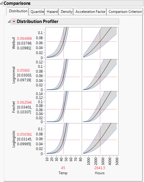
Comparable results appear on the Quantile, Hazard, and Density tabs. The Distribution, Quantile, Hazard, Density, and Acceleration Factor Profilers behave similarly to the Prediction Profiler in other platforms. For example, the vertical lines of Temp and Hours can be dragged to see how each of the distribution values change with temperature and time. For a detailed explanation of the Prediction Profiler, see the Profiler chapter in the Profilers book.
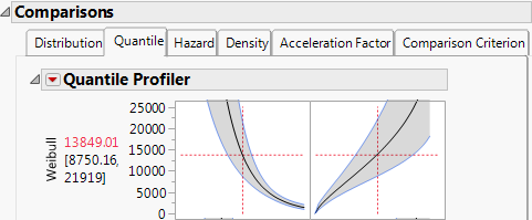
Quantile
You can use the Quantile profiler for extrapolation. Suppose that the data are represented by a Weibull distribution. From viewing the Weibull Acceleration Factor Profiler in Figure 4.11, you see that the acceleration factor at 45 degrees Celsius is 17.18683 for a baseline temperature of 10 degrees Celsius. Select the Quantile tab to see the Quantile Profiler for the Weibull distribution. Select and drag the vertical line in the probability plot so that the probability reads 0.5. From viewing Figure 4.10, where the Probability is set to 0.5, you find that the quantile for the failure probability of 0.5 at 45 degrees Celsius is 13849.01 hours. So, at 10 degrees Celsius, you can expect that 50% of the units fail by 13849.01 * 17.18683 = 238021 hours.
Figure 4.10 Weibull Quantile Profiler for Devalt.jmp
Acceleration Factor
Selecting the Acceleration Factor tab shows the Acceleration Factor Profiler for the time-to-event variable for each specified distribution. To produce Figure 4.11, select Fit All Distributions from the Fit Life by X red triangle menu. Modify the baseline value for the explanatory variable by selecting Set Time Acceleration Baseline from the Fit Life by X red triangle menu and entering the desired value. Note that the explanatory variable and the baseline value appear beside the profiler title.
Figure 4.11 Acceleration Factor Profiler for Devalt.jmp
The Acceleration Factor Profiler lets you estimate time-to-failure for accelerated test conditions when compared with the baseline condition and a parametric distribution assumption. The interpretation of a time-acceleration plot is generally the ratio of the pth quantile of the baseline condition to the pth quantile of the accelerated test condition. This relation applies only when the distribution is Lognormal, Weibull, Loglogistic, or Fréchet, and the scale parameter is constant for all levels. This relation does not apply for a Normal, SEV, Logistic, or LEV distribution.
Note: The Acceleration Factor Profiler does not appear in the following instances: when the explanatory variable is discrete; the explanatory variable is treated as discrete; a customized formula does not use a unity scale factor; or the distribution is Normal, SEV, Logistic, or LEV.
Comparison Criterion
The Comparison Criterion tab shows the -2Loglikelihood, AICc, and BIC criteria for the distributions of interest. Figure 4.12 shows these values for the Weibull, Lognormal, Loglogistic, and Fréchet distributions. Distributions providing better fits to the data are shown at the top of the Comparisons report, sorted by AICc.
Figure 4.12 Comparison Criterion Report Tab
This report suggests that the Lognormal and Loglogistic distributions provide the best fits for the data, because the lowest criteria values are seen for these distributions. For a detailed explanation of the criteria, see “Parametric Distributions” in the “Life Distribution” chapter.
Results
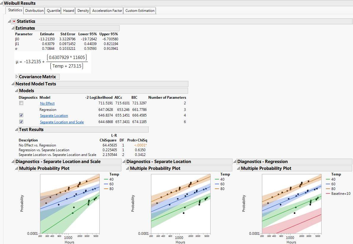
The Results section of the report window shows more detailed statistics and prediction profilers than those shown in the Comparisons report. Separate result sections are shown for each selected distribution. Figure 4.13 shows a portion of the Weibull results, Nested Model Tests, and Diagnostics plots for Devalt.jmp.
Statistical results, diagnostic plots, and Distribution, Quantile, Hazard, Density, and Acceleration Factor Profilers are included for each of your specified distributions. The Custom Estimation tab lets you estimate specific failure probabilities and quantiles, using both Wald and Profile interval methods. When the Box-Cox Relationship is selected on the platform launch window, the Sensitivity tab appears. This tab shows how the Loglikelihood and B10 Life change as a function of Box-Cox lambda.
Figure 4.13 Weibull Distribution Nested Model Tests for Devalt.jmp Data
Statistics
For each parametric distribution, there is a Statistics section that shows parameter estimates, a covariance matrix, confidence intervals, summary statistics, and diagnostic plots. You can save probability, quantile, and hazard estimates by selecting any or all of these options from the Statistics red triangle menu for each parametric distribution. The estimates and the corresponding lower and upper confidence limits are saved as columns in your data table. Figure 4.14 shows the save options available for any parametric distribution.
Figure 4.14 Save Options for Parametric Distribution
Nested Model Tests
Nested Model Tests are included, if you selected the option on the platform launch window. The Nested Model Tests include statistics and diagnostic plots for the following models:
Separate Location and Scale
Assumes that the location and scale parameters are different for all levels of the explanatory variable and is equivalent to fitting the distribution by the levels of the explanatory variable. The Separate Location and Scale Model has multiple location parameters and multiple scale parameters. See Figure 4.15.
Separate Location
Assumes that the location parameters are different, but the scale parameters are the same for all levels of the explanatory variable. The Separate Location Model has multiple location parameters and only one scale parameter. See Figure 4.16.
Regression
Is the default model shown in the initial Fit Life by X report window. See Figure 4.17.
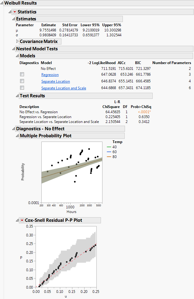
No Effect
Assumes that the explanatory variable does not affect the response and is equivalent to fitting all of the data values to the selected distribution. The No Effect Model has one location parameter and one scale parameter. See Figure 4.18.
Separate Location and Scale, Separate Location, and Regression analyses results are shown by default. Regression parameter estimates and the location parameter formula are shown under the Estimates section, by default. The Diagnostics plots for the No Effect model can be displayed by selecting the check box to the left of No Effect under the Nested Model Tests title.
To see results for each of the models (independently of the other models), click the underlined model of interest (listed under Nested Model Tests) and then uncheck the check boxes for the other models.
If the Nested Model Tests option was not checked in the launch window, then the Separate Location and Scale, and Separate Location models are not assessed. In this case, estimates are given for the regression model for each distribution that you select, and the Cox-Snell Residual P-P Plot is the only diagnostic plot.
Diagnostics
The Multiple Probability Plots shown in Figure 4.13 are used to validate the distributional assumption for the different levels of the accelerating variable. If the line for each level does not run through the data points for that level, the distributional assumption might not hold. Side-by-side comparisons of the diagnostic plots provide a visual comparison for the validity of the different models. See Meeker and Escobar (1998, sec. 19.2.2) for a discussion of multiple probability plots.
The Cox-Snell Residual P-P Plots are used to validate the distributional assumption for the data. If the data points deviate far from the diagonal, then the distributional assumption might be violated. The Cox-Snell Residual P-P Plot red triangle menu has an option called Save Residuals that enables you to save the residual data to the data table. See Meeker and Escobar (1998, sec. 17.6.1) for a discussion of Cox-Snell residuals.
Figure 4.15 Separate Location and Scale Model with the Weibull Distribution for Devalt.jmp Data
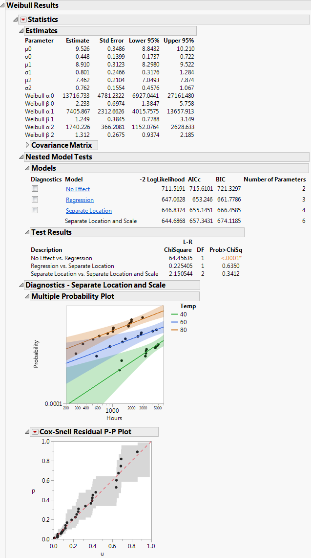
Figure 4.16 Separate Location Model with the Weibull Distribution for Devalt.jmp Data

Figure 4.17 Regression Model with the Weibull Distribution for Devalt.jmp Data
Figure 4.18 No Effect Model with the Weibull Distribution for Devalt.jmp Data
Profilers and Surface Plots
In addition to a statistical summary and diagnostic plots, the Fit Life by X report window also includes profilers and surface plots for each of your specified distributions. To view the Weibull time-accelerating factor and explanatory variable profilers, click the Distribution tab under Weibull Results. To see the surface plot, click the disclosure icon to the left of the Weibull title (under the profilers). The profilers and surface plot behave similarly to other platforms. See the Profiler chapter and the Surface Plot chapter in the Profilers book.
The report window also includes a tab labeled Acceleration Factor. Clicking the Acceleration Factor tab shows the Acceleration Factor Profiler. This profiler is an enlargement of the Weibull plot shown under the Acceleration Factor tab in the Comparisons section of the report window. Figure 4.19 shows the Acceleration Factor Profiler for the Weibull distribution of Devalt.jmp. The baseline level for the explanatory variable can be modified by selecting the Set Time Acceleration Baseline option in the Fit Life by X red triangle menu.
Figure 4.19 Weibull Acceleration Factor Profiler for Devalt.jmp
Custom Relationship
If you want to use a custom transformation to model the relationship between the lifetime event and the accelerating factor, use the Custom option. This option is found in the list under Relationship in the launch window. Enter comma delimited values into the entry fields for the location (μ) and scale (σ) parameters. For the Devalt.jmp sample data, an example entry for μ could be “1, log(:Temp), log(:Temp)^2,” and an entry for σ could be “1, log(:Temp),” where 1 indicates that an intercept is included in the model. Select the Use Exponential Link check box to ensure that the sigma parameter is positive.
Figure 4.20 Custom Relationship Specification in Fit Life by X Launch Window
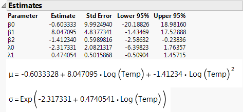
After selecting OK, location and scale transformations are created and included at the bottom of the Estimates report section.
Figure 4.21 Weibull Estimates and Formulas for Custom Relationship
For an example of how to use a custom transformation, see “Custom Relationship Example”. Analysis proceeds similarly to the “Example of the Fit Life by X Platform”, where the Arrhenius Celsius Relationship was specified.
Fit Life by X Platform Options
The following options are accessed by clicking the Fit Life by X red triangle menu in the report window:
Fit Lognormal
Fits a lognormal distribution to the data.
Fit Weibull
Fits a Weibull distribution to the data.
Fit Loglogistic
Fits a loglogistic distribution to the data.
Fit Fréchet
Fits a Fréchet distribution to the data.
Fit Exponential
Fits an exponential distribution to the data.
Fit SEV
Fits an SEV distribution to the data.
Fit Normal
Fits a normal distribution to the data.
Fit Logistic
Fits a logistic distribution to the data.
Fit LEV
Fits an LEV distribution to the data.
Fit All Distributions
Fits all distributions to the data.
Set Time Acceleration Baseline
Enables you to enter a baseline value for the explanatory variable of the acceleration factor in a pop-up dialog.
Change Confidence Level
Lets you enter a desired confidence level, for the plots and statistics, in a pop-up dialog. The default confidence level is 0.95.
Tabbed Report
Lets you specify how you want the report window displayed. Two options are available: Tabbed Overall Report and Tabbed Individual Report. Tabbed Individual Report is checked by default. You can select one, both or none.
Show Surface Plot
Shows or hides the surface plot for the distribution on and off in the individual distribution results section of the report. The surface plot is shown in the Distribution, Quantile, Hazard, and Density sections for the individual distributions, and it is on by default.
Show Points
Shows or hides the data points on and off in the Nonparametric Overlay plot and in the Multiple Probability Plots. The points are shown in the plots by default. If this option is unchecked, step functions are shown instead.
Scatterplot
Shows a scatterplot of a lifetime event versus an explanatory variable.
See the JMP Reports chapter in the Using JMP book for more information about the following options:
Local Data Filter
Shows or hides the local data filter that enables you to filter the data used in a specific report.
Redo
Contains options that enable you to repeat or relaunch the analysis. In platforms that support the feature, the Automatic Recalc option immediately reflects the changes that you make to the data table in the corresponding report window.
Save Script
Contains options that enable you to save a script that reproduces the report to several destinations.
Save By-Group Script
Contains options that enable you to save a script that reproduces the platform report for all levels of a By variable to several destinations. Available only when a By variable is specified in the launch window.
Additional Examples of the Fit Life by X Platform
This section contains additional examples using the Fit Life by X platform.
Capacitor Example
This example uses Capacitor ALT.jmp and can be found in the Reliability folder of the sample data. It contains simulated data that gives censored observations for three levels of temperature, for a reliability study. Observations are shown as censored values at temperature levels of 85, 105, and 125 degrees Celsius.
1. Select Help > Sample Data Library and open Reliability/Capacitor ALT.jmp.
2. Select Analyze > Reliability and Survival > Fit Life by X.
3. Select Hours and click Y, Time to Event.
4. Select Temperature and click X.
5. Select Censor and click Censor.
6. Leave the Censor Code as 1.
7. Select Freq as Freq.
8. Keep Arrhenius Celsius as the relationship, and keep the Nested Model Tests option selected.
9. Select Weibull as the distribution.
10. Keep Wald as the confidence interval method.
Figure 4.22 shows the completed launch window.
Figure 4.22 Fit Life by X Launch Window
11. Click OK.
Figure 4.23 shows the top half of the Fit Life by X report window.
Figure 4.23 Fit Life by X Report Window for Capacitor ALT.jmp Data
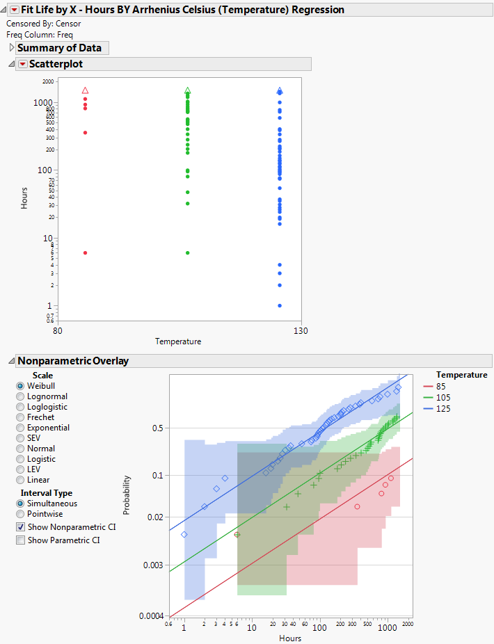
The report window shows summary data, diagnostic plots, comparison data and results, including detailed statistics and prediction profilers. Separate result sections are shown for each selected distribution. Distribution, Quantile, Hazard, Density, and Acceleration Factor Profilers are included for each of the specified distributions.
Custom Relationship Example
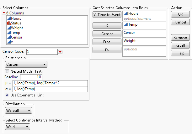
To create a quadratic model with Log(Temp) for the Weibull location parameter and a log-linear model with Log(Temp) for the Weibull scale parameter, follow these steps:
1. Select Help > Sample Data Library and open Reliability/Devalt.jmp.
2. Select Analyze > Reliability and Survival > Fit Life by X.
3. Select Hours and click Y, Time to Event, Temp and click X, Censor and click Censor, and Weight and click Freq.
4. Select Custom as the Relationship from the list.
5. In the entry field for μ, enter 1, log(:Temp), log(:Temp)^2.
(The 1 indicates that an intercept is included in the model.)
6. In the entry field for σ, enter 1, log(:Temp).
7. Select the check box for Use Exponential Link.
8. Deselect the check box for Nested Model Tests.
9. In the entry field for Baseline, enter 10.
10. Select Weibull as the Distribution.
Figure 4.24 shows the completed launch window using the Custom option.
Note: The Nested Model Tests check box is not checked for non-constant scale models. Nested Model test results are not supported for this option.
11. Click OK.
Figure 4.24 Custom Relationship Specification in Fit Life by X Launch Window
Figure 4.25 shows the location and scale transformations, which are subsequently created and included at the bottom of the Estimates report section.
Analysis proceeds similarly to the “Example of the Fit Life by X Platform”, where the Arrhenius Celsius Relationship was specified.
Figure 4.25 Weibull Estimates and Formulas for Custom Relationship
..................Content has been hidden....................
You can't read the all page of ebook, please click here login for view all page.