
Fit Parametric Survival Overview
Survival times can be expressed as a function of one or more variables. When this is the case, use a regression platform that fits a linear regression model while taking into account the survival distribution and censoring. The Fit Parametric Survival platform fits the time to event Y (with censoring) using linear regression models that can involve both location and scale effects. The fit is performed using the Weibull, lognormal, exponential, Fréchet, and loglogistic distributions.
Example of Parametric Regression Survival Fitting
The data table Comptime.jmp contains data on the analysis of computer program execution time whose lognormal distribution depends on the effect Load.
Note: The data in Comptime.jmp comes from Meeker and Escobar (1998, p. 434).
1. Select Help > Sample Data Library and open Reliability/Comptime.jmp.
2. Select Analyze > Reliability and Survival > Fit Parametric Survival.
3. Select ExecTime and click Time to Event.
4. Select Load and click Add.
5. Change the Distribution from Weibull to Lognormal.
6. Click Run.
Figure 14.2 Computing Time Output
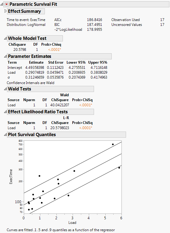
When there is only one effect, a plot of the survival quantiles for three survival probabilities are shown as a function of the effect.
Time quantiles are desired for when 90% of jobs are finished under a system load of 5. See Meeker and Escobar, p. 438.
7. From the red triangle menu, select Estimate Time Quantile.
8. Type 5 as the Load.
9. Type 0.1 as the Survival Prob.
10. Click Go.
Figure 14.3 Estimates of Time Quantile
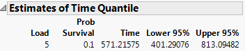
The report estimates that 90% of the jobs will be done by 571 seconds of execution time under a system load of 5.
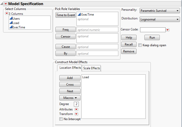
Launch the Fit Parametric Survival Platform
Launch the Fit Parametric Survival platform by selecting Analyze > Reliability and Survival > Fit Parametric Survival.
Figure 14.4 The Fit Parametric Survival Launch Window
Tip: To change the alpha level, click on the red triangle menu and select Set Alpha Level.
Time to Event
Contains the time to event or time to censoring. With interval censoring, specify two Y variables, where one Y variable gives the lower limit and the other Y variable gives the upper limit for each unit.
Censor
Specify a column with indicators to identify right-censored observations. Select the value that identifies right-censored observations from the Censor Code menu. The Censor column is used only when one Time to Event column is entered.
Freq
Specify a column whose values are the frequencies or counts of observations for each row when there are multiple units recorded.
Cause
Specify a column containing multiple failure causes. This column is particularly useful for estimating competing causes. A separate parametric fit is performed for each cause value. Failure events can be coded with either numeric or categorical (labels) values.
By
Performs a separate analysis for each level of a classification or grouping variable.
Location and Scale Effects
Specify location and scale effects using these options. For more information about the Construct Model Effects options, see the Model Specification chapter in the Fitting Linear Models book.
Personality
Indicates the fitting method. Parametric Survival should always be selected.
Distribution
Choose the desired response distribution that is appropriate for your data. Choose the All Distributions option to fit all the distributions and compare the fits. If you choose All Distributions, the report shows a comparison of the distribution fits. See “The Parametric Survival - All Distributions Report”.
Note: By default, the All Distributions option fits a model for the log-location-scale distributions that appear above All Distributions in the Distribution menu. Select Preferences > Platforms > Fit Parametric Survival > Include location-scale distributions in All Distributions to change the behavior of the All Distributions option to also include the location-scale distributions.
Censor Code
After selecting the Censor column, select the value that designates right-censored observations from the list. Missing values are excluded from the analysis. JMP attempts to detect the censor code and display it in the list.
The Parametric Survival Fit Report
If you select All Distributions in the launch window, a Parametric Survival Fit report appears for each distribution. If you specify a Cause column in the launch window, a Parametric Survival Fit report appears for each cause. Otherwise, only one Parametric Survival Fit report appears. Each Parametric Survival Fit report contains the following:
Effect Summary
Shows an interactive report that enables you to add or remove effects from the model. See the Standard Least Squares chapter in the Fitting Linear Models book.
Model Fit Details
The Time to event shows which Y column is specified, and the Distribution shows which distribution is fit. AICc, BIC, and -2*LogLikelihood are all measures of the model fit. These measures allow for comparisons to other model fits. Observation Used and Uncensored Values are summary statistics for the data.
Whole Model Test
Compares the complete fit with an intercept-only fit. If there is only an intercept term, the fit is the same as that from the Life Distribution platform.
Parameter Estimates
Shows the estimates of the regression parameters.
‒ The model has no scale effects.
‒ No Cause column is specified in the launch window.
‒ The Distribution specified in the launch window is Normal, Lognormal, or Weibull.
Alternate Parameterization
(Available only for the Weibull distribution.) Shows the parameter estimates for the α and β parameterization of the Weibull distribution. For more information about this parameterization, see “Weibull” in the “Life Distribution” chapter.
Wald Tests
Shows a Wald Chi-square test for each term in the model.
Effect Likelihood Ratio Tests
Compare the log-likelihood from the fitted model to one that removes each term from the model individually.
Plot Survival Quantiles
Shows the data points plotted with the 0.1, 0.5, and 0.9 quantiles.
Figure 14.5 The Parametric Survival Fit Report
The Parametric Survival - All Distributions Report
The Parametric Survival - All Distributions report appears only when you select All Distributions in the launch window. By default, this report contains a Model Comparison report and Distribution Overlay plot. The Quantile Function Overlay plot is available in the red triangle menu next to Parametric Survival - All Distributions.
Model Comparison
Table that lists fit statistics (AICc and BIC) for the fitted distributions. The distributions with the smallest AICc and BIC values are labeled in the right-most column. If one distribution has the smallest value for both AICc and BIC, that distribution is labeled “Best”. The Parametric Survival Fit report corresponding to the distribution with the smallest AICc is open by default. For more information about these statistics, see the Statistical Details appendix in the Fitting Linear Models book.
Distribution Overlay
Plot of overlaid distribution functions for the fitted distributions at specified values of the effects.
Quantile Function Overlay
Plot of overlaid quantile functions for the fitted distributions at specified values of the effects.
Both the Distribution Overlay and Quantile Function Overlay plots show curves for each of the fitted distributions overlaid on the same graph. By default, each curve has a shaded Wald-based confidence interval. To the right of each plot, there is legend, an option to show shading of confidence intervals, and controls that enable you to specify different values of the effects. Figure 14.6 shows an example of a Distribution Overlay plot.
Note: The alpha level for the shaded confidence intervals can be modified from the launch window. 95% is the default setting.
Figure 14.6 Distribution Overlay Plot

Parametric Competing Cause Report
If you specify a Cause column in the launch window, the Parametric Competing Cause report appears. If you also specify All Distributions in the launch window, this report is labeled Parametric Competing Cause - All Distributions. The Parametric Competing Cause report contains the following:
Summary by Cause
Table that lists fit statistics (AICc and BIC) for each cause. If All Distributions is selected for the Distribution option in the launch window, this table includes fit statistics for each cause within each distribution fit.
Model Comparison
(Available only when All Distributions is selected for the Distribution option in the launch window.) Shows a table that lists fit statistics (AICc and BIC) for the fitted distributions. The distributions with the smallest AICc and BIC values are labeled in the right-most column. If one distribution has the smallest value for both AICc and BIC, that distribution is labeled “Best”. The Parametric Survival Fit report corresponding to the distribution with the smallest AICc is open by default.
For more information about the AICc and BIC statistics, see the Statistical Details appendix in the Fitting Linear Models book.
Fit Parametric Survival Options
The red triangle menu next to Parametric Survival Fit contains the following options:
Likelihood Ratio Tests
Produces tests that compare the log-likelihood from the fitted model to one that removes each term from the model individually.
Wald Tests
Produces chi-square test statistics and p-values for Wald tests of whether each parameter is zero.
Likelihood Confidence Intervals
Specifies the type of confidence intervals shown in the Parameter Estimates table for each parameter. When this option is selected, a profile likelihood confidence interval appears. Otherwise, a Wald interval is shown. In the report, the interval type is noted below the Parameter Estimates table. This option is on by default when the computational time for the profile likelihood confidence intervals is not large.
Note: The alpha level can be modified from the launch window. 95% is the default setting.
Correlation of Estimates
Produces a correlation matrix for the model effects with each other and with the parameter of the fitting distribution.
Covariance of Estimates
Produces a covariance matrix for the model effects with each other and with the parameter of the fitting distribution.
Estimate Survival Probability
Specify effect values and one or more time values. JMP then calculates the survival and failure probabilities with 95% confidence limits for all possible combinations of the entries.
Estimate Time Quantile
Specify effect values and one or more survival values. JMP then calculates the time quantiles and 95% confidence limits for all possible combinations of the entries.
Note: For the Estimate Survival Probability and Estimate Time Quantile options, you can change the alpha level from the default of 95%.
Residual Plot
Shows a probability plot of the standardized residuals.
Save Residuals
Saves the residuals to a new column in the data table.
Distribution Profiler
Shows the response surfaces of the failure probability versus individual explanatory and response variables.
Quantile Profiler
Shows the response surfaces of the response variable versus the explanatory variable and the failure probability.
Distribution Plot by Level Combinations
Shows three probability plots for assessing model fit. The plots show different lines for each combination of the X levels.
Separate Location
is a probability plot assuming equal scale parameters and separate location parameters. This is useful for assessing the parallelism assumption.
Separate Location and Scale
is a probability plot assuming different scale and location parameters. This is useful for assessing if the distribution is adequate for the data. This plot is not shown for the Exponential distribution.
Regression
is a probability plot for which the distribution parameters are functions of the X variables.
Save Probability Formula
Saves the estimated probability formula to a new column in the data table.
Save Quantile Formula
Saves the estimated quantile formula to a new column in the data table. Selecting this option displays a pop-up dialog, asking you to enter a probability value for the quantile of interest.
Model Dialog
Relaunches the launch window.
Effect Summary
Shows the interactive Effect Summary report that enables you to add or remove effects from the model. See the Effect Summary Report section in the Fitting Linear Models book.
Nonlinear Parametric Survival Models
Use the Nonlinear platform for survival models in the following instances:
• The model is nonlinear.
• You need a distribution other than Weibull, lognormal, exponential, Fréchet, or loglogistic.
• You have censoring that is not the usual right, left, or interval censoring.
With the ability to estimate parameters in specified loss functions, the Nonlinear platform becomes a powerful tool for fitting maximum likelihood models. For complete information about the Nonlinear platform, see the Nonlinear Regression chapter in the Predictive and Specialized Modeling book.
To fit a nonlinear model when data are censored, you must first use the formula editor to create a parametric equation that represents a loss function adjusted for censored observations. Then use the Nonlinear platform to estimate the parameters using maximum likelihood.
Additional Examples of Fitting Parametric Survival
This section contains additional examples using the Fit Parametric Survival platform.
Arrhenius Accelerated Failure LogNormal Model
In the Devalt.jmp data, units are stressed by heating, in order to make them fail soon enough to obtain enough failures to fit the distribution.
Note: The data in Devalt.jmp comes from Meeker and Escobar (1998, p. 493).
1. Select Help > Sample Data Library and open Reliability/Devalt.jmp.
First, use the Bivariate platform to see a plot of hours by temperature using the log scale for time.
2. Select Analyze > Fit Y by X.
3. Select Hours and click Y, Response.
4. Select Temp and click X, Factor.
5. Click OK.
Figure 14.7 Bivariate Plot of Hours by Log Temp
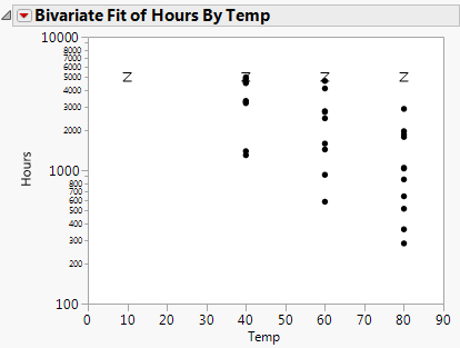
Next, use the survival platform to produce a LogNormal plot of the data for each temperature.
6. Select Analyze > Reliability and Survival > Survival.
7. Select Hours and click Y, Time to Event.
8. Select Censor and click Censor.
9. Select Temp and click Grouping.
10. Select Weight and click Freq.
11. Click OK.
12. From the red triangle menu, select LogNormal Plot and LogNormal Fit.
Figure 14.8 Lognormal Plot

Next, use the Fit Parametric Survival platform to fit one model using an effect for temperature.
13. Select Analyze > Reliability and Survival > Fit Parametric Survival.
14. Select Hours and click Time to Event.
15. Select x and click Add.
16. Select Censor and click Censor.
17. Select Weight and click Freq.
18. Change the Distribution type to Lognormal.
19. Click Run.
Figure 14.9 Devalt Parametric Output
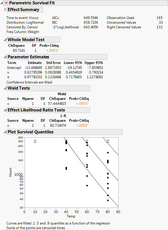
The result shows the regression fit of the data:
‒ If there is only one effect and it is continuous, then a plot of the survival as a function of the effect is shown. Lines are at 0.1, 0.5, and 0.9 survival probabilities.
‒ If the effect column has a formula in terms of one other column, as in this case, the plot is done with respect to the inner column. In this case, the effect was the column x, but the plot is done with respect to Temp, of which x is a function.
Finally, get estimates of survival probabilities extrapolated to a temperature of 10 degrees Celsius for the times 30000 and 10000 hours.
20. From the red triangle menu, select Estimate Survival Probability.
21. Enter the values shown in Figure 14.10 into the Dialog to Estimate Survival.
The Arrhenius transformation of 10 degrees is 40.9853, the effect value.
Figure 14.10 Estimating Survival Probabilities

22. Click Go.
Figure 14.11 Survival Probabilities
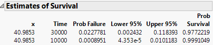
The Estimates of Survival report shows the estimates and a confidence interval.
Interval-Censored Accelerated Failure Time Model
The ICdevice02.jmp data shows failures that were found to have happened between inspection intervals. The model uses two y-variables, containing the upper and lower bounds on the failure times. Right-censored times are shown with missing upper bounds.
Note: The data in ICdevice02.jmp comes from Meeker and Escobar (1998, p. 640).
1. Select Help > Sample Data Library and open Reliability/ICdevice02.jmp.
2. Select Analyze > Reliability and Survival > Fit Parametric Survival.
3. Select HoursL and HoursU and click Time to Event.
4. Select Count and click Freq.
5. Select x and click Add.
6. Click Run.
Figure 14.12 ICDevice Output

The resulting regression shows a plot of time by degrees.
Analyze Censored Data Using the Nonlinear Platform
You can analyze left-censored data using the Nonlinear platform. For the left-censored data, zero is the censored value because it also represents the smallest known time for an observation.
Note: The Tobit model is popular in economics for responses that must be positive or zero, with zero representing a censor point.
Note the following about the Tobit2.jmp data table:
• The response variable is a measure of the durability of a product and cannot be less than zero (Durable, is left-censored at zero).
• Age and Liquidity are independent variables.
• The table also includes the model and tobit loss function. The model in residual form is durable-(b0+b1*age+b2*liquidity). To see the formula associated with Tobit Loss, right-click on the column and select Formula.
Proceed as follows:
1. Select Help > Sample Data Library and open Reliability/Tobit2.jmp.
2. Select Analyze > Specialized Modeling > Nonlinear.
3. Select Model and click X, Predictor Formula.
4. Select Tobit Loss and click Loss.
5. Click OK.
6. Click Go.
7. Click Confidence Limits.
Figure 14.13 Solution Report

Left-Censored Data
The Tobit model is normal and truncated at zero. However, you can take the exponential of the response and set up the intervals for a left-censored problem.
1. Select Help > Sample Data Library and open Reliability/Tobit2.jmp.
2. Select Analyze > Reliability and Survival > Fit Parametric Survival.
3. Select YLow and YHigh and click Time to Event.
4. Select age and liquidity and click Add.
5. Change the Distribution type to Lognormal.
6. Click Run.
Figure 14.14 Tobit Model Results

The report estimates the lognormal model fit.
Weibull Loss Function Using the Nonlinear Platform
In this example, models are fit to the survival time using the Weibull, lognormal, and exponential distributions. Model fits include a simple survival model containing only two effects, a more complex model with all the effects, and the creation of dummy variables for the discrete effect Cell Type to be included in the full model.
Nonlinear model fitting is often sensitive to the initial values that you give to the model parameters. In this example, one way to find reasonable initial values is to first use the Nonlinear platform to fit only the linear model. When the model converges, the solution values for the parameters become the initial parameter values for the nonlinear model.
1. Select Help > Sample Data Library and open VA Lung Cancer.jmp.
The first model and all the loss functions have already been created as formulas in the data table. The Model column has the following formula:
Log(:Time) - (b0 + b1 * Age + b2 * Diag Time)
2. Select Analyze > Specialized Modeling > Nonlinear.
3. Select Model and click X, Predictor Formula.
4. Click OK.
5. Click Go.
Figure 14.15 Initial Parameter Values in the Nonlinear Fit Control Panel
The report computes the least squares parameter estimates for this model.
6. Click Save Estimates.
The parameter estimates in the column formulas are set to those estimated by this initial nonlinear fitting process.
The Weibull column contains the Weibull formula, explained in “Weibull Loss Function”.
To continue with the fitting process:
7. Select Analyze > Specialized Modeling > Nonlinear again.
8. Select Model and click X, Predictor Formula.
9. Select Weibull loss and click Loss.
10. Click OK.
The Nonlinear Fit Control Panel on the left in Figure 14.16 appears. There is now the additional parameter called sigma in the loss function. Because it is in the denominator of a fraction, a starting value of 1 is reasonable for sigma. When using any loss function other than the default, the Loss is Neg LogLikelihood box on the Control Panel is checked by default.
11. Click Go.
The fitting process converges as shown on the right in Figure 14.16.
Figure 14.16 Nonlinear Model with Custom Loss Function

The fitting process estimates the parameters by maximizing the negative log of the Weibull likelihood function.
12. (Optional) Click Confidence Limits to show lower and upper 95% confidence limits for the parameters in the Solution table.
Figure 14.17 Solution Report

Note: Because the confidence limits are profile likelihood confidence intervals instead of the standard asymptotic confidence intervals, they can take time to compute.
You can also run the model with the predefined exponential and lognormal loss functions. Before you fit another model, reset the parameter estimates to the least squares estimates, as they might not converge otherwise. To reset the parameter estimates:
13. (Optional) From the red triangle menu next to Nonlinear Fit, select Revert to Original Parameters.
Fitting Simple Survival Distributions Using the Nonlinear Platform
The following examples show how to use maximum likelihood methods to estimate distributions from time-censored data when there are no effects other than the censor status.
The Loss Function Templates folder has templates with formulas for exponential, extreme value, loglogistic, lognormal, normal, and one-and two-parameter Weibull loss functions. To use these loss functions, copy your time and censor values into the Time and censor columns of the loss function template. To run the model, select Nonlinear and assign the loss column as the Loss variable. Because both the response model and the censor status are included in the loss function and there are no other effects, you do not need a prediction column (model variable).
Exponential, Weibull, and Extreme-Value Loss Function
The Fan.jmp data table can be used to illustrate the Exponential, Weibull, and Extreme value loss functions discussed in Nelson (1982). The data are from a study of 70 diesel fans that accumulated a total of 344,440 hours in service. The fans were placed in service at different times. The response is failure time of the fans or run time, if censored.
Tip: To view the formulas for the loss functions, in the Fan.jmp data table, right-click the Exponential, Weibull, and Extreme value columns and select Formula.
1. Select Help > Sample Data Library and open Reliability/Fan.jmp.
2. Select Analyze > Specialized Modeling > Nonlinear.
3. Select Exponential and click Loss.
4. Click OK.
5. Make sure that the Loss is Neg LogLikelihood check box is selected.
6. Click Go.
7. Click Confidence Limits.
8. Repeat these steps, but select Weibull and Extreme value instead of Exponential.
Figure 14.18 Nonlinear Fit Results

Lognormal Loss Function
The Locomotive.jmp data can be used to illustrate a lognormal loss. The lognormal distribution is useful when the range of the data is several powers of e.
Tip: To view the formula for the loss function, in the Locomotive.jmp data table, right-click on the logNormal column and select Formula.
The lognormal loss function can be very sensitive to starting values for its parameters. Because the lognormal distribution is similar to the normal distribution, you can create a new variable that is the natural log of Time and use Distribution to find the mean and standard deviation of this column. Then, use those values as starting values for the Nonlinear platform. In this example, the mean of the natural log of Time is 4.72 and the standard deviation is 0.35.
1. Select Help > Sample Data Library and open Reliability/Locomotive.jmp.
2. Select Analyze > Specialized Modeling > Nonlinear.
3. Select logNormal and click Loss.
4. Click OK.
5. Click Go.
6. Click Confidence Limits.
Figure 14.19 Solution Report
The maximum likelihood estimates of the lognormal parameters are 5.11692 for Mu and 0.7055 for Sigma (in natural logs). The corresponding estimate of the median of the lognormal distribution is the antilog of 5.11692 (e5.11692), which is approximately 167. This represents the typical life for a locomotive engine.
Statistical Details for Fit Parametric Survival
This section contains statistical details for the Fit Parametric Survival platform.
Loss Formulas for Survival Distributions
The following formulas are for the negative log-likelihoods to fit common parametric models. Each formula uses the calculator if conditional function with the uncensored case of the conditional first and the right-censored case as the Else clause. You can copy these formulas from tables in the Loss Function Templates folder in Sample Data and paste them into your data table.
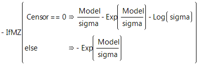
Exponential Loss Function
In the exponential loss function shown here, sigma represents the mean of the exponential distribution and Time is the age at failure.
Exponential Loss Function

A characteristic of the exponential distribution is that the instantaneous failure rate remains constant over time. This means that the chance of failure for any subject during a given length of time is the same regardless of how long a subject has been in the study.
Weibull Loss Function
The Weibull density function often provides a good model for the lifetime distributions. You can use the Survival platform for an initial investigation of data to determine whether the Weibull loss function is appropriate for your data.
Weibull Loss Function
There are examples of one-parameter, two-parameter, and extreme-value functions in the Loss Function Templates folder.
Lognormal Loss Function
The formula shown below is the lognormal loss function where Normal Distribution(model/sigma) is the standard normal distribution function. The hazard function has value 0 at t = 0, increases to a maximum, and then decreases. The hazard function approaches zero as t becomes large.
Lognormal Loss Function

Loglogistic Loss Function
If Y is distributed as the logistic distribution, Exp(Y) is distributed as the loglogistic distribution.
Loglogistic Loss Function

..................Content has been hidden....................
You can't read the all page of ebook, please click here login for view all page.