
The Repairable Systems Simulation (RSS) platform enables you to simulate a repairable system and to analyze its outage time. Outage time is the total time a system is not in the On state as a result of either planned maintenance or unintentional failure.
A repairable system is represented by a system diagram. Block shapes in the system diagram represent one or more components that connect to other components. A component that is performing work in the block is said to be functional. Components can be connected in series or in parallel. When components are connected in series, the system fails if any of the components in the series fails. When components are connected in parallel, the system fails if all of the parallel components fail.
A component pathway is said to be uninterrupted when at least one path between the Start and End blocks does not pass through a block shape failure. During a simulation, the system remains in the On state as long as there is an uninterrupted component pathway. If a block shape failure interrupts the component pathway, the system is set to the Down state. If a block shape fails but the component pathway is not interrupted, the system remains in the On state.
You can add unique events and actions to characterize the repairable nature of individual components. An event is a specific occurrence within the system, such as component failure, scheduled maintenance, or the start of a simulation iteration. Events trigger the execution of one or more actions, which express how components behave. Actions can alter the state of a component or the entire system.
In this example, you run 100 iterations of a simulation of a car system and analyze the system’s estimated outage time over the course of 10 years.
1. Select Help > Sample Data, click Open the Sample Scripts Directory, and open Car Repair Simulation.jsl.
Figure 12.2 Car Repair System Diagram
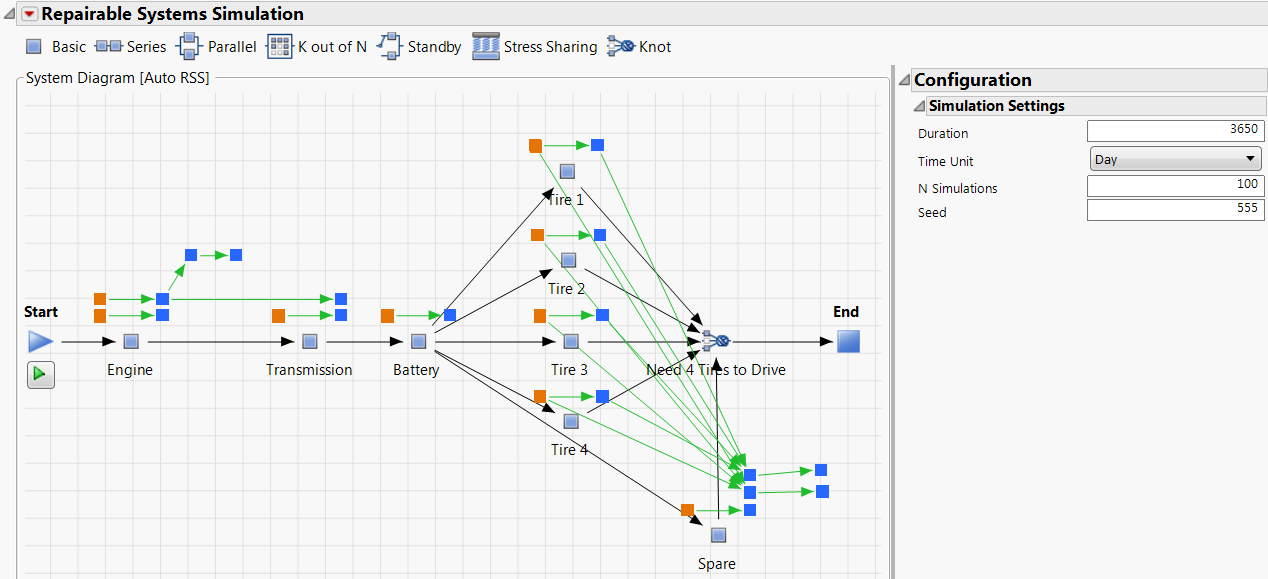
An RSS window that diagrams a car system appears. In the diagram, the first block on the left is the Start block. Notice in the Configuration panel, on the right side of the RSS window, that the simulation is set to run for 3650 days.
2. (Optional) Enter 555 next to Seed.
Because the simulation involves random component failures, this action ensures that you obtain the exact results shown below.
3. Click the green triangle below the Start block to simulate the car system.
A data table that contains the simulation results appears.
4. Click the green arrow next to the Launch Repairable Systems Simulation Results Explorer script.
A window appears containing the Repairable Systems Simulation Results report. For more information about how to interpret these results, see “Repairable Systems Simulation Results”.
Figure 12.3 Partial RSS Report
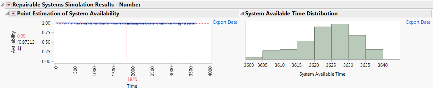
You predict that the car will be available between 3,600 and 3,640 days over the next 10 years. Because the values shown in the Point Estimation of System Availability graph are close to one, you conclude that the car will be mostly available to drive over the next 10 years. You are interested in which components cause the most downtime for the system.
5. Click the red triangle next to Repairable Systems Simulation Results - Number and select Box Plot of Total System Downtime by Component.
Figure 12.4 Partial Box Plot of Total System Downtime by Component Report
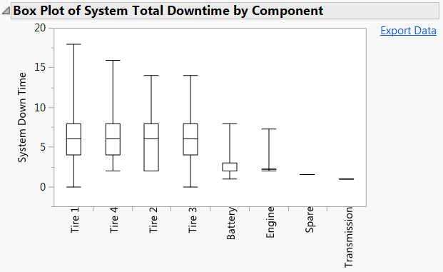
You conclude that the tires cause the most downtime for the car system. To increase the average total system availability, you might consider using more durable tires or carrying another spare tire.
Launch the Repairable Systems Simulation platform by selecting Analyze > Reliability and Survival > Repairable Systems Simulation. The Repairable Systems Simulation window is divided into the following panels:
Figure 12.5 The Repairable Systems Simulation Window
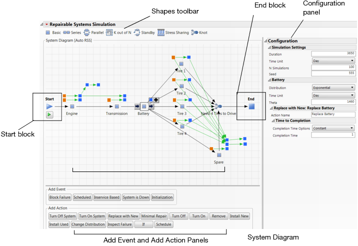
The System Diagram is the space where you can diagram a repairable system. A new System Diagram contains a Start block and an End block.
Tip: To show the Preview window, right-click in the System Diagram and select Diagram Operation > Preview.
The Shapes toolbar contains the block shapes used to represent components in the System Diagram. Add block shapes to the System Diagram by clicking the icon for the block shape and dragging it onto the System Diagram. The Shapes toolbar includes the following block shape icons:
Adds a single block shape that represents a single component.
Adds a series block shape that represents a group of identical components that are connected in series. All of the components must be functional for the block to remain functional.
Adds a parallel block shape that represents a group of identical components that are connected in parallel. At least one of the components must be functional for the block to remain functional.
Adds a k-out-of-n block shape that represents a group of n identical components that are connected in parallel. At least k of the n components must be functional for the block to remain functional.
Adds a standby block shape that represents a group of n identical components that are connected in parallel. Only k components are active, or performing work in the system. The remaining inactive components act as standby components that are activated when any of the k active components fail. The block must have at least k functional and activated components for the block to remain functional.
Adds a stress sharing block shape that represents n identical components that are connected in parallel. Components fail one at a time, and remaining components fail at a quicker rate. The block must have at least one functional component and the block must successfully reallocate stress across remaining components for the block to remain functional.
Adds a knot block shape that represents a combination of the block shapes that point to the knot. At least a specified number of the block shapes that point to the knot must be functional for the knot to remain functional.
For information about the settings available for block shapes, see “Configuration Panel”.
The Simulation Settings report appears at the top of the Configuration panel. The component settings for every selected component appear below the Simulation Settings outline. Configuration settings for selected events and actions appear below the block shape to which the action or event belongs.
Alter the settings for the simulation in the Simulation Settings report, which is available in the Configuration panel. The following settings are available:
Duration
The length of time that is simulated in each iteration.
Time Unit
The unit of time to use for the simulation.
Note: Recurring events and non-immediate actions use the Time Unit specified in Simulation Settings.
N Simulations
The number of iterations in the simulation.
Seed
(Optional) A random seed that ensures the reproducibility of simulation results. By default, the Seed is set to missing, which does not produce reproducible results. When you save the analysis to a script, the random seed that you enter is saved to the script.
Caution: If you run a simulation by right-clicking and selecting Run Multithreaded Simulation, the results are not reproducible, even if you specify a random seed.
Select a block shape in the System Diagram to see its settings in the Configuration panel.
Each block shape, except the knot block, has a failure distribution that determines the rate at which the block shape’s individual components randomly fail. The failure distribution for a basic block determines the rate at which the block fails, because basic blocks represent only one component. For more information about the available failure distribution options, see “Distribution Options”.
Series and Parallel
A series block fails when one of its components fails. A parallel block fails when all of its components fail. The following option is available for series and parallel blocks:
N
Specifies the number of identical components contained in the block.
K-out-of-N
K-out-of-N blocks contain n identical components. The block fails when less than k of the components are functional. The following options are available for K-out-of-N blocks:
K
Specifies the minimum number of functional components required for the block to remain functional.
N
Specifies the number of identical components contained in the block.
Standby
Standby blocks have secondary components, called standby components, that are inactive. Active components perform work within a standby block. Inactive components do not perform work within a standby block, and are activated one at a time as active components fail. Occasionally, the activation process is not successful. A component switch might fail when activating a standby component. A standby block fails when less than k of its n identical components are active. The following options are available for standby blocks:
K
Specifies the number of components that are initially active. This is also the minimum number of active components that is required for the block to remain functional.
N
Specifies the total number of identical components within the block. The difference between k and n is equal to the number of standby components.
Switch Type
Specifies the mechanism that activates a single standby component if any active component fails.
Single Switch
A single switch exists in the block. If the activation of a standby component fails, then the block also fails.
Individual Switches
A switch exists for each standby component. If the activation of a standby component fails, that standby component cannot be activated. The standby block attempts to activate the next standby component until a standby component is activated. If no remaining switches are functional and fewer than k of the components are active, then the block fails.
Switch Reliability
Specifies the probability of success of activating a standby component when any active component fails.
Standby Type
Specifies the state and failure distribution of the standby components.
Cold
Standby components do not age until they are activated.
Warm
Standby components age according to a secondary failure distribution while they are inactive. When standby components are activated, they age according to the primary failure distribution. Use the secondary failure distribution to mimic reduced stress on standby components that are not performing work in the standby block.
Stress Sharing
A stress sharing block distributes stress equally among its components. As components fail, the components that remain functional experience increased stress and subsequently fail at an increased rate.
N
Specifies the total number of identical components contained in the block.
Switch Reliability
Specifies the probability of successfully reallocating stress among the remaining functional components. The block fails if the reallocation of stress fails.
Stress Sharing Type
Specifies how stress is shared among functional components.
Basic (default)
Specifies that stress is shared equally among the remaining functional components. This type of stress sharing is referred to as Load Sharing. The characteristic life of individual components is proportional to the number of components that share the work load.
Custom
Specifies that components share stress according to the JSL code that appears in the Sharing Formula option. The Sharing Formula defines how stress changes when components fail.
Knot
Knot blocks do not have a failure distribution. Knot blocks fail only if the number of connected blocks shapes that are functional falls below the specified minimum number. The following option is available for knot blocks:
Minimum Available
Specifies the minimum number of functional blocks that must point to the knot block for the knot block to remain functional.
Events represent discrete occurrences in a simulation. You can use events to trigger actions. There is no limit to how many actions a single event can trigger. The following options are available in the Add Event Panel:
Note: Some block shapes do not have all of the available event types.
Block Failure
Occurs when the block fails. If the component pathway is interrupted, the system is set to the Down state.
Scheduled
Occurs at a specified recurring interval. The Max Occurrence option sets a limit on the number of occurrences of this event in a simulation. By default, Max Occurrence is set to missing. In this case, the event continues to occur until the end of the simulation. See “Event Settings”.
Inservice Based
Occurs when the component reaches a specified age. A component’s age is the cumulative time that it has been functional and active. Age stops increasing when a component fails or its block is turned off. The Max Occurrence sets a limit on how many times this event can take place in a simulation. By default, the event continues to occur until the end of the simulation. See “Event Settings”.
System is Down
Occurs when the system is set to either the Down or the Off state. The system state can be changed intentionally or unintentionally.
Initialization
Occurs when each simulation iteration begins. Use this event to arrange actions that have to complete before the system runs.
Create an Event
1. To create an event, select a block shape in the System Diagram to display the Add Event and Add Action panels at the bottom of the System Diagram.
2. Select one of the options in the Add Event panel to define an event for the selected block shape.
Figure 12.6 Block Failure Event

An orange square that represents the new event appears above the component. Notice that a connection arrow appears on the right side of the selected event.
An action defines component and system behavior that is triggered by either a connected event or a connected action. Connected actions are triggered upon completion of the prior action. The following options are available in the Add Action Panel:
Note: Some block shapes do not have all of the available action types.
|
Action Name
|
Blocks that can use this Action
|
Starting behavior
|
Completion Behavior
|
|
Turn off System
|
All
|
|
All blocks are turned off. The system is set to the Off state if it was not already in the Down state.
|
|
Turn on System
|
All
|
|
All blocks that were not already failed are turned on. The system is set to the On state if there is an uninterrupted component pathway.
|
|
Replace with New
|
All
|
Turns off the original block, and sets the system to the Down state if the component pathway is interrupted.
|
The block becomes new. Its age is reset and the block is turned on. The system is set to the On state if there is an uninterrupted component pathway.
|
|
Minimal Repair
|
Basic and Series
|
Equivalent to starting behavior for the Replace with New action.
|
Turns the block on.The system is set to the On state if there is an uninterrupted component pathway. The age of the block is not reset.
|
|
Turn On
|
All
|
Cancels the action if the block is in the Down state or is currently removed from the system.
|
Turns the block on increments Turn On Count by one.
|
|
Turn Off
|
All
|
|
Turns the block off. The system is set to the Down state if the component pathway is interrupted.
|
|
Remove
|
All
|
|
The block is removed from the system. The system is set to the Down state if the component pathway is interrupted.
|
|
Install New
|
All
|
Equivalent to starting behavior for Replace with New action.
|
Turns the block off. The age of the block is reset.
|
|
Install Used
|
Basic
|
Equivalent to starting behavior for Replace with New action.
|
Turns the block off. You specify a new age and failure distribution for the block.
|
|
Change Distribution
|
Basic
|
Turns the block off. The system is set to the Down state if the component pathway is interrupted.
|
Changes the failure distribution of the block. Use this to mimic operation changes over time or cumulative damage to the block.
|
|
Inspect Failure
|
All
|
|
Triggers connected actions if the block has failed or is removed from the system.
|
|
If
|
All
|
|
Triggers connected actions if the specified condition script is true.
|
|
Schedule
|
All
|
|
Triggers connected actions at a specified interval. You can limit the number of scheduled intervals or allow the action to continue through the end of the simulation iteration.
|
Create an Action
1. To create an action, select a block shape in the System Diagram to display the Add Event and Add Action panels at the bottom of the System Diagram.
2. Select one of the options from the Add Action panel to define an action for the selected block shape.
A blue action square is created above the selected block shape. Actions are triggered when a connected event occurs. Create an event that triggers the action that you defined.
3. Select one of the options from the Add Event panel to define an event for the selected block shape.
An orange event square is created above the block shape. Notice the connection arrow on the right side of the event.
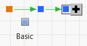
4. Click the connection arrow and drag it to the blue action square that you created in step 2.
A green arrow connects the event and action squares. When the event occurs in a simulation iteration, it triggers the connected action.
5. Select the blue action square that you created in step 2.
You can connect additional actions that are triggered upon completion of the previous action by using the addition sign that appears on the right side of the selected action.
6. Click the addition sign and drag it to an empty area in the System Diagram.
A list of the available actions appears.
7. Select one of the options from the action list to create an action that is connected to the first action.
Figure 12.7 Create an Action
A green arrow connects the two actions. The second action is triggered upon completion of the first action.
The Repairable Systems Simulation red triangle menu contains the following options:
Save and Save As
Enables you to save a Repairable Systems Simulation to a JMP Scripting Language (JSL) script that is automatically executed when it is opened in JMP. See the Getting Started chapter in the Scripting Guide for more information about Auto-Submit scripts.
Note: The Save and Save As red triangle options are equivalent to selecting File > Save and File > Save As, respectively. They are available in the red triangle menu for convenience.
To view settings for the components in a selected design or subsystem, do the following:
• To view the Configuration settings for a block shape, select the block shape in the System Diagram.
• To view Configuration settings for more than one block shape, select multiple block shapes using the Arrow tool, press Control, and click multiple block shapes.
Each block shape randomly fails according to its specified failure distribution. In addition, you specify a time unit for the distribution. The block shape’s time unit can be different from the time unit option that you specify in the simulation settings. The Turn On Count option is based on the number of times the individual block shape has been set to the On state.
The following failure distributions are available:
|
Property Type
|
Required Inputs
|
|
Exponential
|
Theta
|
|
Weibull
|
Alpha, Beta
|
|
Lognormal
|
location, scale
location, scale
location, scale
|
|
Loglogistic
|
|
|
Fréchet
|
|
|
GenGamma
|
mu, sigma, lambda
|
|
DS Weibull
|
Alpha, Beta, Defective Probability
|
|
DS Lognormal
|
location, scale, Defective Probability
location, scale, Defective Probability
location, scale, Defective Probability
|
|
DS Loglogistic
|
|
|
DS Fréchet
|
|
|
Nonparametric
|
data or data file
|
|
Estimated
|
estimated distribution, data or data file
|
To see the formulas and parameterization for these failure distributions, see “Distributions” in the “Life Distribution” chapter.
The Nonparametric and Estimated options under Distribution enable you to approximate an arbitrary distribution. You can enter data manually or import a file that contains data. These data are used to approximate the distribution.
After selecting Nonparametric or Estimated, click the  icon next to Data. The Provide Data window appears, which enables you to either enter data or import a data file. After you have imported or entered your data, the data are used to calculate a distribution for the component.
Figure 12.8 Provide Data Window
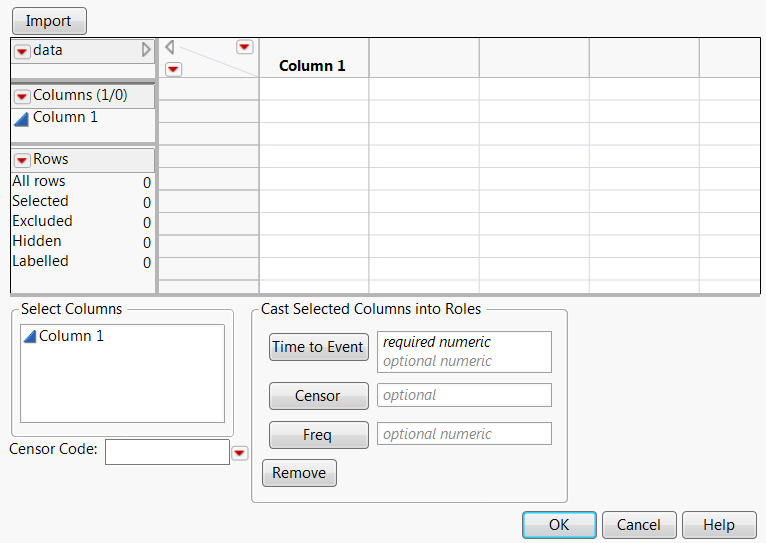
To import data from a file, do the following:
1. Before clicking the icon, open the JMP data table that contains the data to import.
2. Click the icon next to Data.
3. In the Provide Data window, click Import.
The Select Data Table window appears.
4. From the Data Table list, select a data table.
5. Click OK.
6. In the panel beneath the data grid, specify the columns that represent Time to Event data.
7. Specify Censor and Freq columns, if appropriate.
8. In the Provide Data window, click OK.
To enter data manually, do the following:
1. Create columns for Time to Event data.
2. Create columns for Censor and Freq data, if appropriate.
3. Enter the data in the columns.
4. In the panel beneath the data grid, specify which columns represent Time to Event data, as well as Censor and Freq data if appropriate. See step 5 and step 6 above.
5. In the Provide Data window, click OK.
Select an event in the System Diagram to see its settings in the Configuration panel. You can change the Event Name setting to distinguish the event from others. Only the Scheduled and Inservice events have additional settings, which are listed here:
Scheduled
Scheduled events have the following options:
Recurring Interval
Specifies the length of the time interval between event occurrences.
Max Occurrences
Specifies the maximum number of times this event can occur.
Inservice
Inservice events have the following options:
Inservice
Specifies the interval of component run time to wait before this event occurs.
Note: Component run time accumulates only when the system is in the On state and the component is functional.
Max Occurrences
Specifies the maximum number of times this event can occur.
Select an action in the System Diagram to see its settings in the Configuration panel. You can change the Action Name setting to distinguish the action from others. By default, actions are completed immediately. Non-immediate completion time options are available in the Completion Time Options menu.
Figure 12.9 Action Settings

The following options appear in the Completion Time Options list:
Immediate (default)
Specifies that no time passes between starting and completion behavior.
Constant
Specifies that the time lapse is always the specified Completion Time.
Choice
Specifies that the time lapse is randomly chosen from the specified list of Comma-Separated values.
Uniform
Specifies that the time lapse is randomly chosen from a uniform distribution with the specified Minimum and Maximum.
Triangle
Specifies that the time lapse is randomly chosen from a triangular distribution with the specified Minimum, Mode, and Maximum.
Normal
Specifies that the time lapse is randomly chosen from a normal distribution with the specified Mean and Standard Deviation.
The Repairable Systems Simulation platform produces the following results:
When you click the green arrow under the Start block to run the simulation, the results of the simulation appear in a data table. This table describes the events and subsequent actions that occurred in each simulation iteration.
The results table contains the following columns:
Sim ID
Identifies the simulation iteration to which the event or action belongs.
Time
Gives the exact time that the event or action took place in the simulation.
Subject
Gives the name of the block shape to which the event or action is connected or System in the case of system events and actions.
Predicate
Gives the name of the event or action that took place.
State
Gives the state of the Subject at that exact Time. The initialization and termination of each action are denoted with Start and Finish, respectively.
Note
Gives an additional description of an action. The end of each simulation iteration is denoted with End.
Figure 12.10 RSS Results Table

Notice that the first entry in Figure 12.10 is the start of the Initialization Spare in Trunk action, which has an immediate completion time. The action turns the Spare component off and then finishes while Time is still 0.
The next event that occurs is Tire 2 is Unrepairable when approximately 65 days have passed in the first simulation iteration. In row five, the system is unintentionally set to the Down state because only three tires are functional. The Need 4 Tires to Drive knot requires at least four tires, including the Spare, to be functional. The Tire 2 is Unrepairable event simultaneously triggers the Replace Tire 2 action and the Use Spare action. The Drive with Spare action is triggered in row eleven, and the system is set to the On state.
Notice that Tire 2 failed and was replaced by the Spare at the same time. No time elapsed between the time that the system was set to the Down state and the time that the system was returned to the On state. Because the subsequent actions had an immediate completion time, the Tire 2 is Unrepairable event did not cause any system outage time. The results explorer shows the system outage time that accumulates when actions are non-immediate.
When you click the green arrow next to the Launch Repairable Systems Simulation Results Explorer script in the results data table, a report appears that contains an analysis of the simulation results.
Figure 12.11 Partial RSS Explorer Report
By default, the report contains two types of graphs. The first type of graph, shown on the left side of Figure 12.11, is a point estimate graph. The point estimate graph displays aggregated simulation results on the y-axis plotted against simulation iteration time on the x-axis. The range of the x-axis is the duration that you specify in the simulation settings. The estimated probability of the system being available at a given time is shown in red next to the y-axis. Below the point estimate is a 95% confidence interval for the point estimate.
Tip: To see the point estimation of system availability at a specific time in the simulation iteration, click the red number below the x-axis. Specify a time within the range of the simulation duration and press Enter.
The second type of graph, shown on the right side of Figure 12.11, is a histogram of the system available time from the simulation iterations. The bins in the histograms are representative of one of the following:
• Total simulation time.
• Proportion of the simulation duration.
Tip: Select the Export Data option beside a graph to create a data table with the data that the graph uses.
By default, the report contains the following graphs:
Point Estimation of System Availability
Shows a graph over time of the estimated probability that the system is in the On or the Off state during a simulation iteration.
System Available Time Distribution
Shows a histogram of the total time that the system was available for each simulation iteration.
System Availability Distribution
Shows a histogram of the total time that the system was available for each simulation iteration divided by the duration of the simulation. This distribution is the same as the System Available Time Distribution, except that it is shown as a proportion of the duration of the simulation.
Point Estimation of System In Service Probability
Shows a graph over time of the estimated probability that the system is in the On state during a simulation iteration.
System In Service Time Distribution
Shows a histogram of the total time that the system was in the On state for each simulation iteration.
System In Service Probability Distribution
Shows a histogram of the total time that the system was in the On state for each simulation iteration divided by the duration of the simulation. This distribution is the same as System In Service Time Distribution, except that the distribution is shown as a proportion of the duration of the simulation.
Point Estimation of System Unplanned Outage
Shows a graph over time of the estimated probability that the system is in the Down state during a simulation iteration.
System Unplanned Outage Distribution
Shows a histogram of the total time that the system was in the Down state for each simulation iteration.
System Unplanned Outage Percentage Distribution
Shows a histogram of the total time that the system was in the Down state for each simulation iteration divided by the duration of the simulation. This distribution is the same as System Unplanned Outage Distribution, except that the distribution is shown as a proportion of the duration of the simulation.
The Repairable Systems Simulation Results red triangle menu contains the following options:
Point Estimation of Component Availability
For each block shape in the system diagram, this option shows the following reports.
‒ Point Estimation of Availability
‒ Available Time Distribution
‒ Availability Distribution
‒ Point Estimation of Unplanned Outage
‒ Unplanned Outage Time Distribution
‒ Unplanned Outage Distribution
System Availability by Period
Shows a graph that enables you to examine the average system availability during specified time periods. Use the By Time panel to define the time period as an interval of time. Use the By Event panel to define the time period as a specified number of occurrences of one event. When you click Go, the report shows a bar chart of the average system availability during each period.
Box Plot of System Total Downtime by Component
Shows a box plot of the total time the system was in the Down or Off states caused by individual components. The components are ordered by contribution from the most outage time to the least outage time, similar to a Pareto chart.
Box Plot of System Unplanned Total Outage Time by Component
Shows a box plot of total time the system was in the Down state caused by individual components. The components are ordered by contribution from the most outage time to the least outage time, similar to a Pareto chart.
See the JMP Reports chapter in the Using JMP book for more information about the following options:
Redo
Contains options that enable you to repeat or relaunch the analysis. In platforms that support the feature, the Automatic Recalc option immediately reflects the changes that you make to the data table in the corresponding report window.
Save Script
Contains options that enable you to save a script that reproduces the report to several destinations.
Save By-Group Script
Contains options that enable you to save a script that reproduces the platform report for all levels of a By variable to several destinations. Available only when a By variable is specified in the launch window.
Each point estimation profiler within the Repairable Systems Simulation Results Explorer report has a red triangle menu that contains the following options:
Confidence Intervals
Shows or hides the 95% confidence intervals on the point estimation graphs.
Reset Factor Grid
Opens the Factor Settings window, which enables you to modify the parameters of the point estimation graph. See the Profilers chapter in the Profilers book for more information about setting the factor grid.
Factor Settings
Provides additional options affecting the Factor Grid. See the Profilers chapter in the Profilers book for more information about Factor Settings.
..................Content has been hidden....................
You can't read the all page of ebook, please click here login for view all page.