
Fit Proportional Hazards Overview
The proportional hazards model is a special semiparametric regression model proposed by D. R. Cox (1972) to examine the effect of explanatory variables on survival times. The survival time of each member of a population is assumed to follow its own hazard function.
Proportional hazards is nonparametric in the sense that it involves an unspecified arbitrary baseline hazard function. It is parametric because it assumes a parametric form for the covariates. The baseline hazard function is scaled by a function of the model’s (time-independent) covariates to give a general hazard function. Unlike the Kaplan-Meier analysis, proportional hazards computes parameter estimates and standard errors for each covariate. The regression parameters (β) associated with the explanatory variables and their standard errors are estimated using the maximum likelihood method. A conditional risk ratio (or hazard ratio) is also computed from the parameter estimates.
The survival estimates in proportional hazards are generated using an empirical method. See Lawless (1982). They represent the empirical cumulative hazard function estimates, H(t), of the survivor function, S(t), and can be written as S0 = exp(-H(t)), with the hazard function calculated as follows:

When there are ties in the response, meaning there is more than one failure at a given time event, the Breslow likelihood is used.
Example of the Fit Proportional Hazards Platform
The following example illustrates one nominal effect with two levels. For an example with multiple effects and multiple levels, see “Example Using Multiple Effects and Multiple Levels”.
1. Select Help > Sample Data Library and open Rats.jmp.
2. Select Analyze > Reliability and Survival > Fit Proportional Hazards.
3. Select days and click Time to Event.
4. Select Censor and click Censor.
5. Select Group and click Add.
6. Click Run.
Figure 15.2 Proportional Hazards Fit Report for Rats.jmp Data
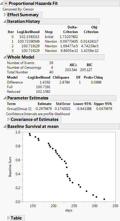
In the Rats.jmp data, there are only two groups. Therefore, in the Parameter Estimates report, a confidence interval that does not include zero indicates an alpha-level significant difference between groups. Also, in the Effect Likelihood Ratio Tests report, the test of the null hypothesis for no difference between the groups shown in the Whole Model Test table is the same as the null hypothesis that the regression coefficient for Group is zero.
Risk Ratios for One Nominal Effect with Two Levels
To show risk ratios for effects, select the Risk Ratios option from the red triangle menu. In this example, there is only one effect, and there are only two levels for that effect. The risk ratio for Group 2 is compared with Group 1 and appears in the Risk Ratios for Group report. See Figure 15.3. The risk ratio in this table is determined by computing the exponential of the parameter estimate for Group 2 and dividing it by the exponential of the parameter estimate for Group 1.
Note the following:
• The Group 1 parameter estimate appears in the Parameter Estimates table. See Figure 15.2.
• The Group 2 parameter estimate is calculated by taking the negative value for the parameter estimate of Group 1.
• Reciprocal shows the value for 1/Risk Ratio.
Tip: To see the Reciprocal values, right-click in the Risk Ratios report and select Columns > Reciprocal.
For this example, the risk ratio for Group2/Group1 is calculated as follows:
exp[-(-0.2979479)] /exp(-0.2979479) = 1.8146558
This risk ratio value suggests that the risk of death for Group 2 is 1.81 times higher than that for Group 1.
Figure 15.3 Risk Ratios for Group Table

For information about calculating risk ratios when there are multiple effects, or categorical effects with more than two levels, see “Risk Ratios for Multiple Effects and Multiple Levels”.
Launch the Fit Proportional Hazards Platform
Launch the Fit Proportional Hazards platform by selecting Analyze > Reliability and Survival > Fit Proportional Hazards.
Figure 15.4 The Fit Proportional Hazards Launch Window
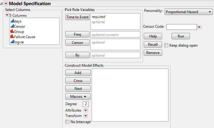
Time to Event
Contains the time to event or time to censoring.
Censor
Nonzero values in the censor column indicate censored observations. (The coding of censored values is usually equal to 1.) Uncensored values must be coded as 0.
Freq
Column whose values are the frequencies or counts of observations for each row when there are multiple units recorded.
By
Performs a separate analysis for each level of a classification or grouping variable.
Construct Model Effects
Enters effects into your model. For more details about the Construct Model Effects options, see the Model Specification chapter in the Fitting Linear Models book.
Personality
Indicates the fitting method. Proportional Hazard should always be selected.
Censor Code
Enter the value of the Censor column that corresponds to a censored observation.
The Fit Proportional Hazards Report
Finding parameter estimates for a proportional hazards model is an iterative procedure. When the fitting is complete, the report in Figure 15.5 appears.
Figure 15.5 The Proportional Hazards Fit Report
Iteration History
Lists iteration results occurring during the model calculations.
Whole Model
Shows the negative of the natural log of the likelihood function (–LogLikelihood) for the model with and without the covariates. Twice the positive difference between them gives a chi-square test of the hypothesis that there is no difference in survival time among the effects. The degrees of freedom (DF) are equal to the change in the number of parameters between the full and reduced models.
Parameter Estimates
Shows the parameter estimates for the covariates, their standard errors, and 95% upper and lower confidence limits. A confidence interval for a continuous column that does not include zero indicates that the effect is significant. A confidence interval for a level in a categorical column that does not include zero indicates that the difference between the level and the average of all levels is significant.
Effect Likelihood Ratio Tests
Shows the likelihood ratio chi-square test of the null hypothesis that the parameter estimates for the effects of the covariates is zero.
Baseline Survival at mean
Plots the baseline function estimates at each event time in the data. The values in the Table report are plotted here.
Fit Proportional Hazards Options
The red triangle next to Proportional Hazards Fit contains the following options:
Likelihood Ratio Tests
Produces tests that compare the log-likelihood from the fitted model to one that removes each term from the model individually.
Wald Tests
Produces chi-square test statistics and p-values for Wald tests of whether each parameter is zero.
Likelihood Confidence Intervals
Specifies the type of confidence intervals shown in the Parameter Estimates table for each parameter. When this option is selected, a profile likelihood confidence interval appears. Otherwise, a Wald interval is shown. In the report, the interval type is noted below the Parameter Estimates table. This option is on by default when the computational time for the profile likelihood confidence intervals is not large.
Note: The alpha level can be modified from the launch window. 95% is the default setting.
Risk Ratios
Shows the risk ratios for the effects. For continuous columns, unit risk ratios and range risk ratios are calculated. The Unit Risk Ratio is Exp(estimate) and the Range Risk Ratio is Exp[estimate*(xMax – xMin)]. The Unit Risk Ratio shows the risk change over one unit of the regressor, and the Range Risk Ratio shows the change over the whole range of the regressor. For categorical columns, risk ratios are shown in separate reports for each effect. Note that for a categorical variable with k levels, only k -1 design variables, or levels, are used.
Tip: To see Reciprocal values in the Risk Ratio report, right-click in the report and select Columns > Reciprocal.
Model Dialog
Shows the completed launch window for the current analysis.
Effect Summary
Shows the interactive Effect Summary report that allows you to add or remove effects from the model. See the Effect Summary Report section in the Fitting Linear Models book.
Example Using Multiple Effects and Multiple Levels
This example uses a proportional hazards model for the sample data, VA Lung Cancer.jmp. The data were collected from a randomized clinical trial, where males with inoperable lung cancer were placed on either a standard or a novel (test) chemotherapy (Treatment). The primary interest of this trial was to assess if the treatment type has an effect on survival time, with special interest given to the type of tumor (Cell Type). See Prentice (1973) and Kalbfleisch and Prentice (2002) for additional details about this data set.
For the proportional hazards model, covariates include the following:
• Whether the patient had undergone previous therapy (Prior)
• Age of the patient (Age)
• Time from lung cancer diagnosis to beginning the study (Diag Time)
• A general medical status measure (KPS)
Age, Diag Time, and KPS are continuous measures and Cell Type, Treatment, and Prior are categorical (nominal) variables. The four nominal levels of Cell Type include Adeno, Large, Small, and Squamous.
This example illustrates the results for a model with more than one effect and a nominal effect with more than two levels. Risk ratios are also demonstrated, with example calculations for risk ratios for a continuous effect and risk ratios for an effect that has more than two levels.
1. Select Help > Sample Data Library and open VA Lung Cancer.jmp.
2. Select Analyze > Reliability and Survival > Fit Proportional Hazards.
3. Select Time as Time to Event.
4. Select censor as Censor.
5. Select Cell Type, Treatment, Prior, Age, Diag Time, and KPS and click Add.
6. Click Run.
7. From the red triangle menu, select Risk Ratios.
8. (Optional) Click the disclosure icon on the Baseline Survival at mean title bar to close the plot, and click the disclosure icon on Whole Model to close the report.
Figure 15.6 Report Window for Proportional Hazards Model with Multiple Effects and Levels
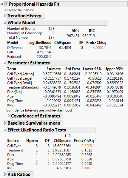
Note the following about the results:
• In the Whole Model report, the low Prob>Chisq value (<.0001) indicates that there is a difference in survival time when at least one of the effects is included in the model.
• In the Effect Likelihood Ratio Tests report, the Prob>ChiSq values indicate that KPS and at least one of the levels of Cell Type are significant, while Treatment, Prior, Age, and Diag Time effects are not significant.
Risk Ratios for Multiple Effects and Multiple Levels
Figure 15.6 shows the Risk Ratios for the continuous effects (Age, Diag Time, KPS) and the nominal effects (Cell Type, Treatment, Prior). For illustration, focus on the continuous effect, Age, and the nominal effect with four levels (Cell Type) for the VA Lung Cancer.jmp sample data.
For the continuous effect, Age, in the VA Lung Cancer.jmp sample data, the risk ratios are calculated as follows:
Unit Risk Ratios
exp(β) = exp(-0.0085494) = 0.991487
Range Risk Ratios
exp[β(xmax - xmin)] = exp(-0.0085494 * 47) = 0.669099
For the nominal effect, Cell Type, all pairs of levels are calculated and are shown in the Risk Ratios for Cell Type table. Note that for a categorical variable with k levels, only k -1 design variables, or levels, are used. In the Parameter Estimates table, parameter estimates are shown for only three of the four levels for Cell Type (Adeno, Large, and Small). The Squamous level is not shown, but it is calculated as the negative sum of the other estimates. Here are two example Risk Ratios for Cell Type calculations:
Large/Adeno = exp(βLarge)/exp(βAdeno) = exp(-0.2114757)/exp(0.57719588) = 0.4544481
Squamous/Adeno = exp[-(βAdeno + βLarge + βSmall)]/exp(βAdeno)
= exp[-(0.57719588 + (-0.2114757) + 0.24538322)]/exp(0.57719588) = 0.3047391
Reciprocal shows the value for 1/Risk Ratio.
..................Content has been hidden....................
You can't read the all page of ebook, please click here login for view all page.