
Survival Analysis Overview
Survival data need to be analyzed with specialized methods for two reasons:
1. The survival times usually have specialized non-normal distributions, like the exponential, Weibull, and lognormal.
2. Some of the data could be censored.
Survival functions are calculated using the nonparametric Kaplan-Meier method for one or more groups of either complete or right-censored data. Complete data have no censored values. Right-censoring is when you do not know the exact survival time, but you know that it is greater than the specified value. Right-censoring occurs when the study ends without all the units failing, or when a patient has to leave the study before it is finished. The censored observations cannot be ignored without biasing the analysis. The elements of a survival model are:
• A time indicating how long until the unit (or patient) either experienced the event or was censored. Time is the model response (Y).
• A censoring indicator that denotes whether an observation experienced the event or was censored. JMP uses the convention that the code for a censored unit is 1 and the code for a non-censored event is zero.
• Explanatory variables (if a regression model is used.)
• Interval censoring is when a data point is somewhere on an interval between two values. If interval censoring is needed, then two Y variables hold the lower and upper limits bounding the event time.
Common terms used for reliability and survival data include lifetime, life, survival, failure-time, time-to-event, and duration.
The Survival platform computes product-limit (Kaplan-Meier) survival estimates for one or more groups. It can be used as a complete analysis or is useful as an exploratory analysis to gain information for more complex model fitting. The Kaplan-Meier Survival platform does the following:
• Shows a plot of the estimated survival function for each group and, optionally, for the whole sample.
• Calculates and lists survival function estimates for each group and for the combined sample.
• Shows exponential, Weibull, and lognormal diagnostic failure plots to graphically check the appropriateness of using these distributions for further regression modeling. Parameter estimates are available on request.
• Computes the Log Rank and generalized Wilcoxon Chi-square statistics to test homogeneity of the estimated survival function across groups.
• Analyzes competing causes, prompting for a cause of failure variable, and estimating a Weibull failure time distribution for censoring patterns corresponding to each cause.
Example of Survival Analysis
An experiment was undertaken to characterize the survival time of rats exposed to a carcinogen in two treatment groups. The data are in the Rats.jmp sample data table. The event in this example is death. The objective is to see whether rats in one treatment group live longer (more days) than rats in the other treatment group.
1. Select Help > Sample Data Library and open Rats.jmp.
The data in the days column is the survival time. Notice that some observations are censored.
2. Select Analyze > Reliability and Survival > Survival.
3. Select days and click Y, Time to Event.
4. Select Group and click Grouping.
5. Select Censor and click Censor.
6. Click OK.
Figure 13.2 Survival Plot for Rats.jmp Data
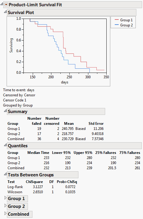
It appears that the rats in treatment group 1 are living longer than the rats in treatment group 2.
Launch the Survival Platform
Launch the Survival platform by selecting Analyze > Reliability and Survival > Survival.
Figure 13.3 The Survival Launch Window

Y, Time to Event
(Required) Contains the time to event or time to censoring. If you have interval censoring, specify two Y variables, representing the lower and upper limits.
Grouping
Classifies the data into groups that are fit separately.
Censor
Identifies censored values. Enter the value that identifies censoring in the Censor Code box. This column can contain more than two distinct values under the following conditions:
‒ All censored rows have the value entered in the Censor Code box.
‒ Non-censored rows have a value other than what is in the Censor Code box.
Freq
Indicates the column whose values are the frequencies of observations for each row when there are multiple units recorded. If the value is 0 or a positive integer, then the value represents the frequencies or counts of observations for each row.
By
Performs a separate analysis for each level of a classification or grouping variable.
Plot Failure instead of Survival
Shows a failure probability plot instead of its reverse (a survival probability plot).
Censor Code
Specify the code that represents censored values.
The Survival Plot
The Survival platform shows overlay step plots of estimated survival functions for each group. A legend identifies groups by color and line type.
Figure 13.4 The Survival Plot

Reports beneath the plot show summary statistics and quantiles for survival times. Estimated survival times for each observation are computed within groups. Survival times are computed from the combined sample. When there is more than one group, statistical tests compare the survival curves.
Survival Platform Options
The red triangle menu next to Product-Limit Survival fit contains the following options:
Survival Plot
Shows the overlaid survival plots for each group.
Failure Plot
Shows the overlaid failure plots (proportion failing over time) for each group (in the tradition of the reliability literature.) A failure plot reverses the y-axis to show the number of failures rather than the number of survivors.
Note: The Failure Plot option replaces the Reverse Y Axis option found in older versions of JMP (which is still available in scripts).
Plot Options
Contains the following options:
Note: The first seven options (Show Points, Show Kaplan Meier, Show Combined, Show Confid Interval, Show Simultaneous CI, Show Shaded Pointwise CI, and Show Shaded Simultaneous CI) and the last two options (Fitted Survival CI, Fitted Failure CI) pertain to the initial survival plot and failure plot. The other five (Midstep Quantile Points, Connect Quantile Points, Fitted Quantile, Fitted Quantile CI Lines, Fitted Quantile CI Shaded) pertain only to the distributional plots.
‒ Show Points shows the sample points at each step of the survival plot. Failures appear at the bottom of the steps, and censorings are indicated by points above the steps.
‒ Show Kaplan Meier shows the Kaplan-Meier curves. This option is on by default.
‒ Show Combined shows the survival curve for the combined groups in the Survival Plot.
‒ Show Confid Interval shows the pointwise 95% confidence bands on the survival plot for groups and for the combined plot when it appears with the Show Combined option.
‒ When you select Show Points and Show Combined, the survival plot for the total or combined sample appears as a gray line. The points also appear at the plot steps of each group.
‒ Show Simultaneous CI shows the simultaneous confidence bands for all groups on the plot. Meeker and Escobar (1998, chap. 3) discuss pointwise and simultaneous confidence intervals and the motivation for simultaneous confidence intervals in survival analysis.
‒ Midstep Quantile Points changes the plotting positions to use the modified Kaplan-Meier plotting positions, which are equivalent to taking mid-step positions of the Kaplan-Meier curve, rather than the bottom-of-step positions. This option is recommended, so it is on by default.
‒ Connect Quantile Points shows the lines in the plot. This option is on by default.
‒ Fitted Quantile shows the straight-line fit on the fitted Weibull, lognormal, or exponential plot. This option is on by default.
‒ Fitted Quantile CI Lines shows the 95% confidence bands for the fitted Weibull, lognormal, or exponential plot.
‒ Fitted Quantile CI Shaded shows the display of the 95% confidence bands for a fit as a shaded area or dashed lines.
‒ Fitted Survival CI shows the confidence intervals (on the survival plot) of the fitted distribution.
‒ Fitted Failure CI shows the confidence intervals (on the failure plot) of the fitted distribution.
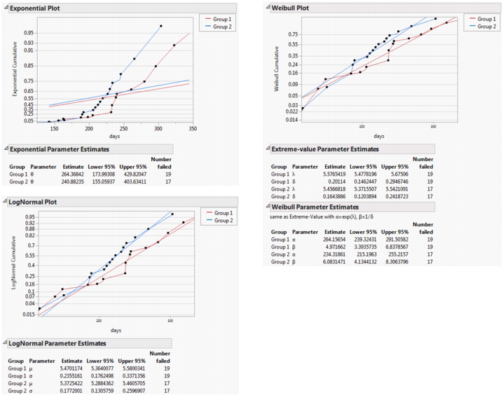
Exponential Plot
Plots the cumulative exponential failure probability by time for each group. Lines that are approximately linear empirically indicate the appropriateness of using an exponential model for further analysis. For example, in Figure 13.5, the lines for Group 1 and Group 2 in the Exponential Plot are curved rather than straight. This indicates that the exponential distribution is not appropriate for this data. See “Exponential, Weibull, and Lognormal Plots and Fits”.
Exponential Fit
Produces the Exponential Parameters table and the linear fit to the exponential cumulative distribution function in the Exponential Plot. See Figure 13.5. The parameter Theta corresponds to the mean failure time. See “Exponential, Weibull, and Lognormal Plots and Fits”.
Weibull Plot
Plots the cumulative Weibull failure probability by log(time) for each group. A Weibull plot that has approximately parallel and straight lines indicates a Weibull survival distribution model might be appropriate to use for further analysis. See “Exponential, Weibull, and Lognormal Plots and Fits”.
Weibull Fit
Produces the linear fit to the Weibull cumulative distribution function in the Weibull plot and two popular forms of Weibull estimates. These estimates are shown in the Extreme-value Parameter Estimates table and the Weibull Parameter Estimates tables. See Figure 13.5. The Alpha parameter is the 0.632 quantile of the failure-time distribution. The Extreme-value table shows a different parameterization of the same fit, where Lambda = ln(Alpha) and Delta = 1/Beta. See “Exponential, Weibull, and Lognormal Plots and Fits”.
LogNormal Plot
Plots the cumulative lognormal failure probability by log(time) for each group. A lognormal plot that has approximately parallel and straight lines indicates a lognormal distribution is appropriate to use for further analysis. See “Exponential, Weibull, and Lognormal Plots and Fits”.
LogNormal Fit
Produces the linear fit to the lognormal cumulative distribution function in the lognormal plot and the LogNormal Parameter Estimates table shown in Figure 13.5. Mu and Sigma correspond to the mean and standard deviation of a normally distributed natural logarithm of the time variable. See “Exponential, Weibull, and Lognormal Plots and Fits”.
Fitted Distribution Plots
Use in conjunction with the fit options to show three plots corresponding to the fitted distributions: Survival, Density, and Hazard. If you have not performed a fit, no plot appears. See “Fitted Distribution Plots”.
Competing Causes
Performs an estimation of the Weibull model using the specified causes to indicate a failure event and other causes to indicate censoring. The fitted distribution appears as a dashed line in the Survival Plot. See “Competing Causes”.
Estimate Survival Probability
Estimates survival probabilities for the time values that you specify.
Estimate Time Quantile
Estimates a time quantile for each survival probability that you specify.
Save Estimates
Creates a data table containing survival and failure estimates, along with confidence intervals, and other distribution statistics.
Exponential, Weibull, and Lognormal Plots and Fits
For each of the three distributions that JMP supports, there is a plot command and a fit command. Use the plot command to see whether the event markers seem to follow a straight line. The markers tend to follow a straight line when the distributional fit is suitable for the data. Then, use the fit commands to estimate the parameters.
Figure 13.5 Exponential, Weibull, and Lognormal Plots and Reports
The following table shows what to plot to make a straight line fit for that distribution:
|
Distribution Plot
|
X Axis
|
Y Axis
|
Interpretation
|
|
Exponential
|
time
|
-log(S)
|
slope is 1/theta
|
|
Weibull
|
log(time)
|
log(-log(S))
|
slope is beta
|
|
Lognormal
|
log(time)
|
Probit(1-S)
|
slope is 1/sigma
|
Note: S = product-limit estimate of the survival distribution.
The exponential distribution is the simplest, with only one parameter, called theta. It is a constant-hazard distribution, with no memory of how long it has survived to affect how likely an event is. The parameter theta is the expected lifetime.
The Weibull distribution is the most popular for event-time data. There are many ways in which different authors parameterize this distribution (as shown in Table 13.2). JMP reports two parameterizations, labeled the lambda-delta extreme value parameterization and the Weibull alpha-beta parameterization. The alpha-beta parameterization is used in the reliability literature. See Nelson (1990). Alpha is interpreted as the quantile at which 63.2% of the units fail. Beta is interpreted as follows: if beta>1, the hazard rate increases with time; if beta<1, the hazard rate decreases with time; and if beta=1, the hazard rate is constant, meaning it is the exponential distribution.
|
JMP Weibull
|
alpha
|
beta
|
|
Wayne Nelson
|
alpha=alpha
|
beta=beta
|
|
Meeker and Escobar
|
eta=alpha
|
beta=beta
|
|
Tobias and Trindade
|
c = alpha
|
m = beta
|
|
Kececioglu
|
eta=alpha
|
beta=beta
|
|
Hosmer and Lemeshow
|
exp(X beta)=alpha
|
lambda=beta
|
|
Blishke and Murthy
|
beta=alpha
|
alpha=beta
|
|
Kalbfleisch and Prentice
|
lambda = 1/alpha
|
p = beta
|
|
JMP Extreme Value
|
lambda=log(alpha)
|
delta=1/beta
|
|
Meeker and Escobar s.e.v.
|
mu=log(alpha)
|
sigma=1/beta
|
The lognormal distribution is also very popular. This is the distribution where if you take the log of the values, the distribution is normal. If you want to fit data to a normal distribution, you can take the exp() of it and analyze it as lognormal. See “Additional Examples of Fitting Parametric Survival” in the “Fit Parametric Survival” chapter.
Additional Options
To see additional options for the exponential, Weibull, and lognormal fits, hold down the Shift key, click the red triangle of the Product-Limit Survival Fit menu, and click on the desired fit.
Use these options to:
• Set the confidence level for the limits.
• Set the constrained value for theta (in the case of an exponential fit), sigma (in the case of a lognormal fit) or beta (in the case of a Weibull fit). See “WeiBayes Analysis”.
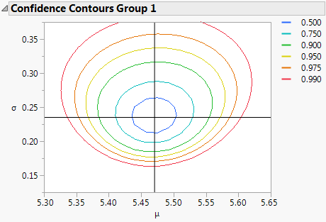
• Obtain a Confidence Contour Plot for the Weibull and lognormal fits (when there are no constrained values). See Figure 13.6.
Figure 13.6 Confidence Contour Plot
WeiBayes Analysis
JMP can constrain the values of the Theta (Exponential), Beta (Weibull), and Sigma (LogNormal) parameters when fitting these distributions. This feature is needed in WeiBayes situations, for example:
• Where there are few or no failures
• There are existing historical values for beta
• There is still a need to estimate alpha
For more details about WeiBayes situations, see Abernethy (1996).
With no failures, the standard technique is to add a failure at the end and the estimates would reflect a type of lower bound on what the alpha value would be, rather than a real estimate. The WeiBayes feature allows for a true estimation.
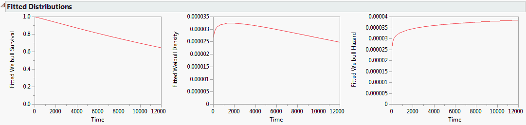
Fitted Distribution Plots
Use the Fitted Distribution Plots option to see Survival, Density, and Hazard plots for the exponential, Weibull, and lognormal distributions. The plots share the same axis scaling so that the distributions can be easily compared.
Figure 13.7 Fitted Distribution Plots for Three Distributions

These plots can be transferred to other graphs through the use of graphic scripts. To copy the graph, right-click in the plot to be copied and select Edit > Copy Frame Contents. Right-click in the destination plot and select Edit > Paste Frame Contents.
Competing Causes
Sometimes there are multiple causes of failure in a system. For example, suppose that a manufacturing process has several stages and the failure of any stage causes a failure of the whole system. If the different causes are independent, the failure times can be modeled by an estimation of the survival distribution for each cause. A censored estimation is undertaken for a given cause by treating all the event times that are not from that cause as censored observations.
The red triangle menu next to Competing Causes contains the following options:
Omit Causes
Removes the specified cause value and recalculates the survival estimates.
Save Cause Coordinates
Adds a new column to the current table called log(–log(Surv)). This information is often used to plot against the time variable with a grouping variable, such as the code for type of failure.
Weibull Lines
Adds Weibull lines to the plot.
Hazard Plot
Adds a Hazard Plot.
Simulate
Creates a new data table containing time and cause information from the Weibull distribution, as estimated by the data.
Additional Examples of Survival Analysis
The failure of diesel generator fans was studied by Nelson (1982, p. 133) and Meeker and Escobar (1998, appendix C1).
1. Select Help > Sample Data Library and open Reliability/Fan.jmp.
2. Select Analyze > Reliability and Survival > Survival.
3. Select Time and click Y, Time to Event.
4. Select Censor and click Censor.
5. Select the check box for Plot Failure instead of Survival.
6. Click OK.
Figure 13.8 Fan Initial Output
Notice that the probability of failure increases over time. Often the next step is to explore distributional fits, such as a Weibull model. From the red triangle menu, select Weibull Plot and Weibull Fit.
Figure 13.9 Weibull Output for Fan Data

Because the fit is reasonable and the Beta estimate is near 1, you can conclude that this looks like an exponential distribution, which has a constant hazard rate. From the red triangle menu, select Fitted Distribution Plots. Three views of the Weibull fit appear.
Figure 13.10 Fitted Distribution Plots
Example of Competing Causes
Nelson (1982) discusses the failure times of a small electrical appliance that has a number of causes of failure. One group (Group 2) of the data is represented in the JMP sample data table Appliance.jmp.
1. Select Help > Sample Data Library and open Reliability/Appliance.jmp.
2. Select Analyze > Reliability and Survival > Survival.
3. Select Time Cycles and click Y, Time to Event.
4. Click OK.
5. From the red triangle menu, select Competing Causes.
6. Click Cause Code, and click OK.
7. From the red triangle menu next to Competing Causes, select Hazard Plot.
Figure 13.11 Competing Causes Report and Hazard Plot
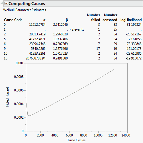
The survival distribution for the whole system is simply the product of the survival probabilities. The Competing Causes table shows the Weibull estimates of Alpha and Beta for each failure cause.
In this example, most of the failures were due to cause 9. Cause 1 occurred only once and could not produce good Weibull estimates. Cause 15 happened for very short times and resulted in a small beta and large alpha. Recall that alpha is the estimate of the 63.2% quantile of failure time, which means that causes with early failures often have very large alphas; if these causes do not result in early failures, then these causes do not usually cause later failures.
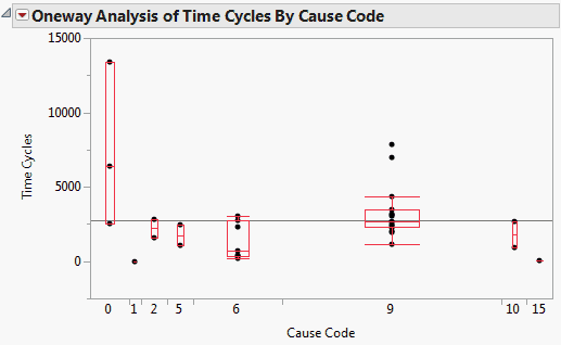
Figure 13.12 shows the Fit Y by X plot of Time Cycles by Cause Code with the Quantiles option in effect. This plot further illustrates how the alphas and betas relate to the failure distribution.
Figure 13.12 Fit Y by X Plot of Time Cycles by Cause Code
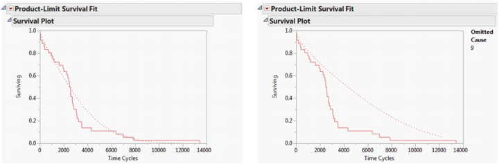
In this example, recall that cause 9 was the source of most of the failures. If cause 9 was corrected, how would that affect the survival due to the remaining causes? Select the Omit Causes option to remove a cause value and recalculate the survival estimates.
Figure 13.13 shows the survival plots with all competing causes and without cause 9. You can see that the survival rate (represented by the dashed line) without cause 9 does not improve much until 2,000 cycles, but then becomes much better and remains improved, even after 10,000 cycles.
Figure 13.13 Survival Plots with Omitted Causes
Example of Interval Censoring
With interval censored data, you know only that the events occurred in some time interval. The Turnbull method is used to obtain nonparametric estimates of the survival function.
In this example from Nelson (1990, p. 147), microprocessor units are tested and inspected at various times and the failed units are counted. Missing values in one of the columns indicate that you do not know the lower or upper limit, and therefore the event is left or right censored, respectively.
1. Select Help > Sample Data Library and open Reliability/Microprocessor Data.jmp.
2. Select Analyze > Reliability and Survival > Survival.
3. Select start time and end time and click Y, Time to Event.
4. Select count and click Freq.
5. Select the check box next to Plot Failure instead of Survival.
6. Click OK.
7. From the red triangle menu, select LogNormal Fit.
Figure 13.14 Interval Censoring Output
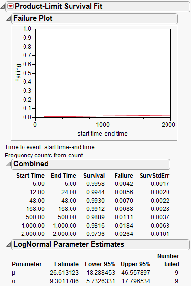
The resulting Turnbull estimates are shown. Turnbull estimates might have gaps in time where the survival probability is not estimable, as seen here between, for example, 6 and 12, 24 and 48, 48 and 168” and so on.
At this point, select a distribution to see its fitted estimates —in this case, a Lognormal distribution is fit. Notice that the failure plot shows very small failure rates for these data.
Statistical Reports for Survival Analysis
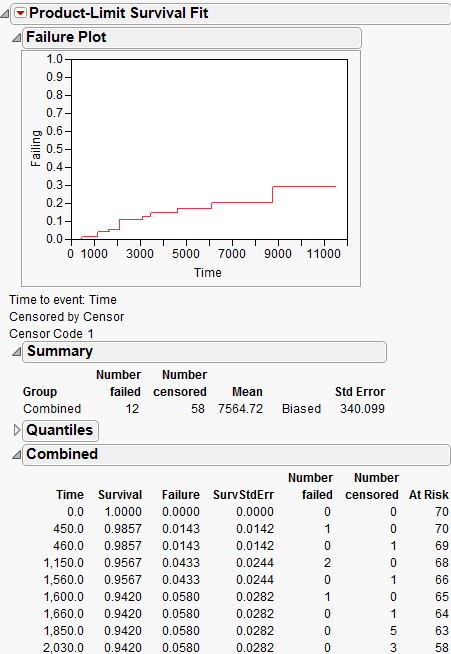
For data that is not interval censored, the initial reports show Summary and Quantiles data (Figure 13.15). The Summary data shows the number of failed and number of censored observations for each group (when there are groups) and for the whole study. The mean and standard deviations are also adjusted for censoring. For computational details about these statistics, see the SAS/STAT User’s Guide (2001).
The Quantiles data shows time to failure statistics for individual and combined groups. These include the median survival time, with upper and lower 95% confidence limits. The median survival time is the time (number of days) at which half the subjects have failed. The quartile survival times (25% and 75%) are also included.
Figure 13.15 Summary Statistics for the Univariate Survival Analysis

The Summary report gives estimates for the mean survival time, as well as the standard error of the mean. The estimated mean survival time is as follows:
 , with a standard error of
  ,
,where  ,
,  , and
, and  .
.
, , and .D is the number of distinct event times
ni is the number of surviving units just prior to ti
di is the number of units that fail at ti
t0 is defined to be 0
When there are multiple groups, the Tests Between Groups table provides statistical tests for homogeneity among the groups. Kalbfleisch and Prentice (1980, chap. 1), Hosmer and Lemeshow (1999, chap. 2), and Klein and Moeschberger (1997, chap. 7) discuss statistics and comparisons of survival curves.
Figure 13.16 Tests between Groups
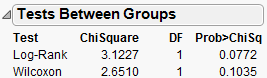
Test
Names two statistical tests of the hypothesis that the survival functions are the same across groups.
Chi-Square
Provides the Chi-square approximations for the statistical tests.
The Log-Rank test places more weight on larger survival times and is more useful when the ratio of hazard functions in the groups being compared is approximately constant. The hazard function is the instantaneous failure rate at a given time. It is also called the mortality rate or force of mortality.
The Wilcoxon test places more weight on early survival times and is the optimum rank test if the error distribution is logistic.(Kalbfleisch and Prentice, 1980).
DF
Provides the degrees of freedom for the statistical tests.
Prob>ChiSq
Lists the probability of obtaining, by chance alone, a Chi-square value greater than the one computed if the survival functions are the same for all groups.
Figure 13.17 shows an example of the product-limit survival function estimates for one of the groups.
Figure 13.17 Example of Survival Estimates Table

Note: When the final time recorded is a censored observation, the report indicates a biased mean estimate. The biased mean estimate is a lower bound for the true mean.
..................Content has been hidden....................
You can't read the all page of ebook, please click here login for view all page.