
Cumulative Damage Platform Overview
A cumulative damage experiment, also called a varying-stress experiment, is an accelerated life test where the stress levels can change over time. The stress can be applied by many different forces: load, temperature, pressure. A typical cumulative damage experiment consists of multiple test units. Each unit has an initial stress level, and the stress level can be changed throughout the experiment.
The most common cumulative damage experiment is a step-stress experiment. A step-stress experiment uses multiple units with varying levels of stress applied. Stress can be applied using factors such as temperature, pressure, or voltage. For each unit, there is an initial stress level. At specified time points, the stress levels are adjusted based on different patterns of stress levels. Between stress level changes, the stress level remains constant.
The Cumulative Damage platform also includes three other varying-stress pattern models:
• In a ramp-stress experiment, the stress levels start at an initial value and then increase linearly over time at a specified slope.
• In a sinusoid-stress experiment, the stress levels fluctuate in a periodic fashion that is defined by a sine wave.
• In a piecewise ramp-stress experiment, the stress levels are defined at specified time points similar to the step-stress case. However, the stress level is not required to stay constant between time points. Rather, it changes linearly from a starting stress level to an ending stress level between time points. If a pair of starting and ending stress levels are equal, the interval is equivalent to a step-stress interval.
For more information about varying-stress and step-stress models, see Nelson (2004, Ch. 10).
Example of the Cumulative Damage Platform
A step-stress experiment is conducted on 40 test units at varying stress conditions. Your goal is to estimate the probability of failure at 10,000 time units given a stress level of 0.75. These data tables are based on data from Nelson (2004, Ch. 10).
The Reliability/CD Step Stress Pattern.jmp data table contains a column called Pattern ID that identifies four different stress patterns. The stress level at a particular step is the ratio of Voltage to Thickness. (Note that these two columns are hidden.) Thickness is held constant for each stress pattern. However, Voltage is set to different levels and increases within each pattern.
The Reliability/CD Step Stress.jmp data table contains the time to failure data.
1. Select Help > Sample Data Library and open Reliability/CD Step Stress.jmp and Reliability/CD Step Stress Pattern.jmp.
The CD Step Stress table contains failure time data:
‒ The Time column gives the failure times.
‒ The Pattern ID column identifies the stress pattern.
‒ The Censor column indicates whether the failure time is exact or censored.
Each row of the table corresponds to one test unit.
The CD Step Stress Pattern table contains the four stress patterns (identified as 1 through 4). The levels of the stress factor, Stress, are varied within each value of the Pattern ID column. The Duration column represents how many time units a particular level of the stress factor lasted.
2. Select Analyze > Reliability and Survival > Cumulative Damage.
The launch window has two sections: one for the failure time data (Time-to-Event) and one for the stress pattern data (Stress Pattern).
3. Click Select Table in the Time-to-Event panel.
A Time-to-Event Data Table window appears, which prompts you to specify the data table for the failure time data.
4. Select CD Step Stress and click OK.
The columns from this table now populate the Select Columns list in the Time-to-Event panel.
5. Select Time and click Time to Event.
6. Select Censor and click Censor.
7. Select Pattern ID for Pattern ID.
8. Click Select Table in the Stress Pattern panel.
9. Select CD Step Stress Pattern and click OK.
The columns from this table now populate the Select Columns list in the Stress Pattern panel.
10. Select Duration and click Stress Duration.
11. Select Stress and click Stress.
12. Select Pattern ID and click Pattern ID.
13. Click OK.
Figure 5.2 Event Plot and Stress Patterns Plot

Figure 5.2 shows the initial report that contains the Event Plot and a plot of the defined stress patterns. All four stress patterns increase the stress level quickly over the first 40 time units, after which they increase at much different rates.
14. Select Fit All from the Cumulative Damage red triangle menu.
Figure 5.3 Model List Report

Figure 5.3 shows the Model List report. From this report, you determine that the best fitting distribution is the Exponential distribution.
15. In the Results report, scroll to the Exponential report.
16. In the Distribution Profiler report, set the current value of Stress to 0.75.
17. Set the current value of Time to 10000.
Figure 5.4 Distribution Profiler for Exponential Distribution at Specified Settings
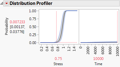
Figure 5.4 shows that the predicted probability of failure for a test unit under constant stress of 0.75 at 10000 time units is 0.007233, with a 95% confidence interval of 0.00137 to 0.03776.
Launch the Cumulative Damage Platform
Launch the Cumulative Damage platform by selecting Analyze > Reliability and Survival > Cumulative Damage. You must supply the Cumulative Damage platform with two data tables as input. The first data table is time-to-event data for each unit under test. The second data table defines the stress patterns used for each unit.
Figure 5.5 Cumulative Damage Launch Window
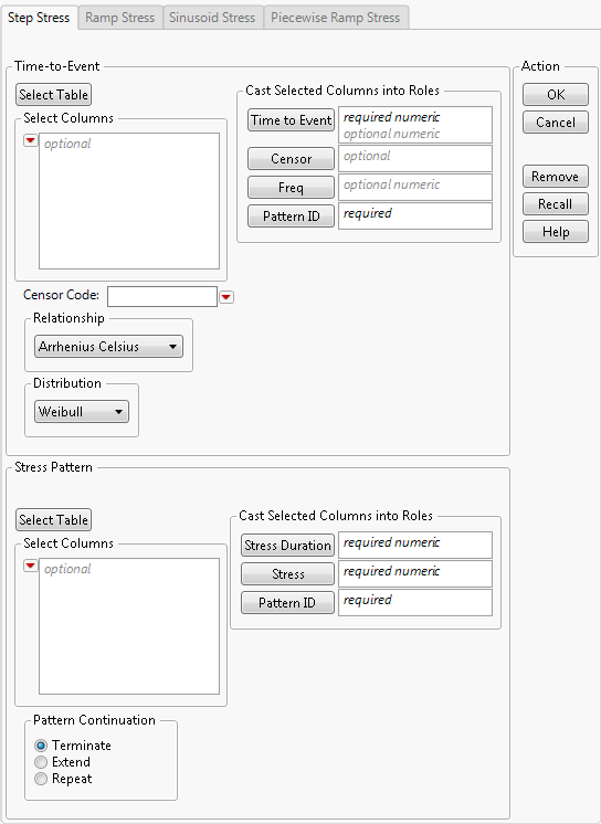
The launch window includes a separate tab for each step-stress data format. For details about the various stress patterns, see “Stress Pattern”.
Each of the step-stress format tabs contains two panels for specifying variables for the model:
• The Time-to-Event panel is common to all of the step-stress formats. This panel is similar to the Fit Life by X platform launch window.
• The Stress Pattern panel is used to describe the type of stress. Consequently, its format depends on the selected step-stress tab.
Time to Event
The Time to Event panel in the Cumulative Damage launch window contains the following options:
Time to Event
Identifies the time to event (such as the time to failure) or time to censoring. For interval censoring, your data table should contain two columns, where one gives the lower bound and the other gives the upper bound of the failure time for each unit. Enter the two censoring columns as Time to Event. For details about censoring, see “Event Plot” in the “Life Distribution” chapter.
Censor
Identifies right-censored observations. Select the value that identifies right-censored observations from the Censor Code menu beneath the Select Columns list. The Censor column is used only when one Y is entered.
Freq
Identifies frequencies or observation counts when there are multiple units. If the value is 0 or a positive integer, then the value represents the frequencies or counts of observations with the given row’s settings.
Pattern ID
Contains values that specify the stress pattern in the Stress Pattern data table that was used for the given row.
Censor Code
After selecting the Censor column, select the value that designates right-censored observations from the list. Missing values are excluded from the analysis. JMP attempts to detect the censor code and display it in the list.
Relationship
Determines the relationship between the event and the stress factor. Table 5.1 defines the model for each relationship.
|
Relationship
|
Model
|
|
Arrhenius Celsius
|
μ = b0 + b1 * 11605 / (X+273.15)
|
|
Arrhenius Fahrenheit
|
μ = b0 + b1 * 11605 / ((X + 459.67)/1.8)
|
|
Arrhenius Kelvin
|
μ = b0 + b1 * 11605/X
|
|
Inverse Power (default)
|
μ = b0 + b1 * log(X)
|
|
Linear
|
μ = b0 + b1* X
|
|
Log
|
μ = b0 + b1 * log(X)
|
|
Logit
|
μ = b0 + b1 * log(X/(1-X))
|
|
Reciprocal
|
μ = b0 + b1/X
|
|
Square Root
|
μ = b0 + b1 * sqrt(X)
|
|
Box-Cox
|
μ = b0 + b1 * BoxCox(X)
|
|
Custom
|
user-defined (Available only in the Step Stress panel.)
|
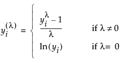
The BoxCox(X) transformation is defined as follows:
If you select Custom, additional controls appear that require you to define the Custom transformation that models the relationship between the lifetime event and the stress factor.
See “Custom Relationship” in the “Fit Life by X” chapter if you want to use a Custom relationship for your model.
Distribution
Specifies an initial time-to-failure distribution. Select from Weibull, Lognormal, Loglogistic, Fréchet, or Exponential. Weibull is the default setting. For more information about the distributions, see “Distributions” in the “Life Distribution” chapter.
Stress Pattern
Specify the stress patterns used in the experiment using the second panel.
Step Stress Pattern
The Step Stress pattern has stress levels that are changed at arbitrary time points. The duration of each stress step and associated stress level must be specified in ascending time order.
The Stress Pattern panel in the Step Stress tab contains the following options:
Stress Duration
The column that contains the length in time units of each stress step.
Stress
The column that contains the level of the stress setting.
Pattern ID
The column that contains a unique identifier for the stress pattern. This column is used to match stress patterns in the Stress Pattern data table with the observations in the Time-to-Event data table.
Pattern Continuation
Specifies how to handle failures that occur after the final time period in the defined stress pattern. This panel contains the following options:
Terminate
A failure that occurs at a time beyond the final time period in the defined stress pattern produces an error, and the model is not fit.
Extend
A failure that occurs at a time beyond the final time period in the defined stress pattern assumes the same stress level as the level in the final time period.
Repeat
A failure that occurs at a time beyond the final time period in the defined stress pattern assumes the same stress level as if the stress pattern were being repeated. For example, if a failure occurs 10 time units after the final time period in the defined stress pattern, then the stress level at that failure time is set to the stress level at 10 time units after the beginning of the defined stress pattern.
Note: The default Pattern Continuation setting for the Step Stress Pattern is Terminate.
Ramp Stress Pattern
The Ramp Stress pattern defines stress as a linear function of time. Each pattern is defined by an intercept (the stress level at time zero) and a slope (the increase in the stress level for every one time unit). Each pattern is described in a single row in the stress pattern data table.
Intercept
The column that contains the intercept for each pattern.
Slope
The column that contains the slope for each pattern.
Pattern ID
The column that contains a unique identifier for the stress pattern. This column is used to match stress patterns in the Stress Pattern data table with the observations in the Time-to-Event data table.
Sinusoid Stress Pattern
The Sinusoid Stress pattern defines stress as a periodic function. The pattern is defined by a level, an amplitude, a period, and a phase. Each pattern is described in a single row in the stress pattern data table. The definition of the pattern is as follows:
S(t) = level + amplitude * sin(phase + (2*π*t) / period)
Level
The column that contains the level for each pattern.
Amplitude
The column that contains the amplitude for each pattern.
Period
The column that contains the period for each pattern.
Phase
The column that contains the phase for each pattern.
Pattern ID
The column that contains a unique identifier for the stress pattern. This column is used to match stress patterns in the Stress Pattern data table with the observations in the Time-to-Event data table.
Piecewise Ramp Stress Pattern
The Piecewise Ramp Stress pattern defines stress as a piecewise linear function of time. The line segments for the stress level over time can be disjoint or continuous. Line segments can also be flat, so that step stress and ramp stress can be combined. The line segments are defined in the stress pattern data table by the time duration of the segment and the start and end levels of the stress setting.
Stress Duration
The column that contains the length in time units of each stress step.
Stress Ramp
The two columns that contain the stress levels at the start and end of the step.
Pattern ID
The column that contains a unique identifier for the stress pattern. This column is used to match stress patterns in the Stress Pattern data table with the observations in the Time-to-Event data table.
Pattern Continuation
The Pattern Continuation panel enables you to specify the stress levels that occur after the final time period in the defined stress pattern. This panel contains the following options:
Terminate
A failure that occurs at a time beyond the final time period in the defined stress pattern produces an error, and the model is not fit.
Extend
A failure that occurs at a time beyond the final time period in the defined stress pattern assumes the same stress level as the level in the final time period.
Repeat
A failure that occurs at a time beyond the final time period in the defined stress pattern assumes the same stress level as if the stress pattern were being repeated. For example, if a failure occurs 10 time units after the final time period in the defined stress pattern, then the stress level at that failure time is set to the stress level at 10 time units after the beginning of the defined stress pattern.
Note: The default Pattern Continuation setting for the Piecewise Ramp Stress Pattern is Terminate.
The Cumulative Damage Report
After you click OK, the Cumulative Damage report window appears. By default, the Cumulative Damage report contains an event plot, a stress patterns report, a model list, and model results.
Event Plot
The Event Plot in Cumulative Damage displays time to failure or censoring. For details, see “Event Plot” in the “Life Distribution” chapter.
Stress Patterns Report
The Stress Patterns report shows a plot of the stress level over time for each of the stress pattern IDs. The Simulate option in this report enables you to simulate new data. Figure 5.6 shows an example of the Stress Patterns report plot. See “Stress Patterns Options”.
Figure 5.6 Stress Patterns Report

Model List
The Model List report provides the -2*LogLikelihood, number of parameters, AICc, and BIC statistics for each fitted distribution. Smaller values of each of these statistics (other than number of parameters) indicate a better fit. For more details about these statistics, see the Statistical Details appendix in the Fitting Linear Models book.
Model Results
The Results report contains a separate report for each fitted distribution. Each report contains the following:
Parameter Estimates
Shows the estimates, standard errors, and Wald-based 95% confidence intervals.
The fitted equation appears below the Parameter Estimates table. This equation takes into account the fitted parameter estimates and the relationship specified in the launch window.
Distribution Profiler
Shows cumulative failure probability as a function of time.
Quantile Profiler
Shows failure time as a function of cumulative probability.
Hazard Profiler
Shows the hazard rate as a function of time.
Density Profiler
Shows the density function for the distribution.
Cox-Snell Residual P-P Plot
Shows a residual plot that is used to validate the distributional assumption for the data.
The Cox-Snell Residual P-P Plot red triangle menu has a Save Residuals option that saves the Cox-Snell residuals to three new columns in the failure time data table. The three columns are Left Residuals, Right Residuals, and Residual Weight. See Meeker and Escobar (1998, sec. 17.6.1) for a discussion of Cox-Snell residuals.
Cumulative Damage Platform Options
The Cumulative Damage red triangle menu contains the following options:
Fit All
Fits the distributions that were not selected in the launch window. The available distributions are listed under “Distribution”.
See the JMP Reports chapter in the Using JMP book for more information about the following options:
Local Data Filter
Shows or hides the local data filter that enables you to filter the data used in a specific report.
Redo
Contains options that enable you to repeat or relaunch the analysis. In platforms that support the feature, the Automatic Recalc option immediately reflects the changes that you make to the data table in the corresponding report window.
Save Script
Contains options that enable you to save a script that reproduces the report to several destinations.
Save By-Group Script
Contains options that enable you to save a script that reproduces the platform report for all levels of a By variable to several destinations. Available only when a By variable is specified in the launch window.
Stress Patterns Options
The Stress Pattern red triangle menu contains the Simulate option, which shows or hides the Simulation Configuration panel.
The Simulation Control Panel
Figure 5.7 shows the Simulation Configuration Panel. The initial values for Distribution and the parameter settings are determined by the parameter estimates for the distribution specified in the Cumulative Damage launch window. The graph shows the estimated failure distribution functions over time for the stress patterns defined in the Stress Pattern data table.
Figure 5.7 Simulation Configuration Panel
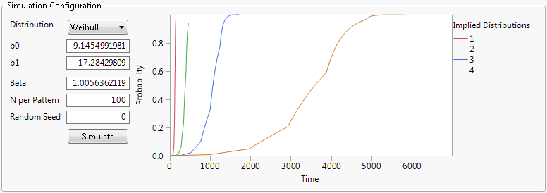
The Simulation Configuration panel enables you to simulate new failure time data based on a distribution and stress pattern. The stress pattern defined in the Stress Pattern data table used in the launch of the platform is also used for the simulation. This panel contains the following options:
Distribution
The distribution to be used for the simulation. The available distributions are the same as in the Cumulative Damage launch window. For more information about the distributions, see “Distributions” in the “Life Distribution” chapter.
b0
The intercept for the location parameter of the distribution.
b1
The slope for the location parameter of the distribution.
lambda
(Available only for the BoxCox relationship.) The lambda value for the BoxCox relationship.
b2, s0, s1, and so on
(Available only for the Custom relationship.) Other parameters that are defined in the Custom relationship in the Cumulative Damage launch window.
Beta
(Available only for the Weibull distribution.) The Beta parameter of the Weibull distribution.
sigma
(Available only for the Lognormal, Loglogistic, and Fréchet distributions.) The sigma parameter of the distribution.
N per Pattern
The number of points generated in the simulation for each stress pattern.
Random Seed
(Optional) A nonzero random seed that ensures the reproducibility of simulation results.
Termination
(Not available when the specified Pattern Continuation in the Cumulative Damage launch window is Terminate.) A time beyond which surviving test units are censored.
Simulate
The plot in the Simulation Configuration panel shows the implied distributions for each of the stress patterns over time. Click the Simulate button to generate a new JMP data table that contains the results of the simulation.
Additional Example of the Cumulative Damage Platform
This section contains additional examples using the Cumulative Damage platform.
Example of Simulating New Data
This example illustrates using the Simulation Configuration panel in the Cumulative Damage report window to generate new step stress data. This example uses the same data as the example in “Example of the Cumulative Damage Platform”.
1. Select Help > Sample Data Library and open Reliability/CD Step Stress.jmp and Reliability/CD Step Stress Pattern.jmp.
2. In the CD Step Stress data table, run the script Cumulative Damage.
3. In the Stress Patterns red triangle menu, select Simulate.
Figure 5.8 Simulation Configuration Panel
The Simulation Configuration panel appears in the Stress Patterns report. The selection for Distribution is Weibull. The fitted values for b0 and b1 are used as initial values for the simulation.
4. Select Exponential for Distribution.
5. Enter 10 for b0.
6. Enter -18 for b1.
7. (Optional) Enter 14678 for Random Seed.
8. Click Simulate.
Figure 5.9 Partial Results of Simulation
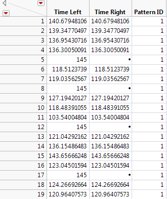
Figure 5.9 shows a partial listing of the simulated data table. The stress pattern with Pattern ID equal to 1 is defined only up to 145 time units. Since the Pattern Configuration setting in the launch window was set to Terminate, the simulation censors any simulated values at 145 for stress pattern 1.
..................Content has been hidden....................
You can't read the all page of ebook, please click here login for view all page.