

Let’s create another game, making full use of loop. But this won’t be a game that we play. Instead, it will be a game world that evolves as we watch it! We’re going to create an environment of steppes and jungles, filled with animals running around, foraging, eating, and reproducing. And after a few million units of time, we’ll see that they’ve evolved into different species!
Note
This example is adapted from A.K. Dewdney’s article “Simulated evolution: wherein bugs learn to hunt bacteria,” in the “Computer Recreations” column of Scientific American (May 1989: 138-141).
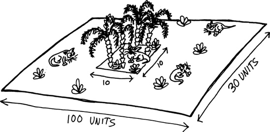
Our game world is extremely simple. It consists of a simple rectangular plane, with edges that wrap around to the opposite side. (Mathematically speaking, it has a toroidal topology.) Most of this world is covered in steppes, meaning that very few plants grow for the animals to eat. In the center of the world is a small jungle, where plants grow much faster. Our animals, who are herbivores, will forage this world in search for food.
Let’s create some variables describing the extent of our world:
(defparameter *width* 100)
(defparameter *height* 30)
(defparameter *jungle* '(45 10 10 10))
(defparameter *plant-energy* 80)
We’re giving the world a width of 100 units and a height of 30 units. Using these dimensions should make it easy to display the world in our Lisp REPL. The *jungle* list defines the rectangle in the world map that contains the jungle. The first two numbers in the list are the x- and y-coordinates of the jungle’s top-left corner, and the last two numbers are its width and height. Finally, we give the amount of energy contained in each plant, which is set to 80. This means that if an animal finds a plant, it will gain 80 days’ worth of food by eating it.
Note
If your terminal window isn’t large enough to display the entire world, change the values of the *width* and *height* variables. Set the *width* variable to the width of your terminal window minus two, and the *height* variable to the height of your terminal window minus one.
As you might imagine, simulating evolution on a computer is a slow process. In order to see the creatures evolve, we need to simulate large stretches of time, which means we’ll want our code for this project to be very efficient. As animals wander around our world, they will need to be able to check if there is a plant at a given x,y location. The most efficient way to enable this is to store all of our plants in a hash table, indexed based on each plant’s x- and y-coordinates.
(defparameter *plants* (make-hash-table :test #'equal))
By default, a Common Lisp hash table uses eq when testing for the equality of keys. For this hash table, however, we’re defining :test to use equal instead of eq, which will let us use cons pairs of x- and y-coordinates as keys. If you remember our rule of thumb for checking equality, cons pairs should be compared using equal. If we didn’t make this change, every check for a key would fail, since two different cons cells, even with the same contents, test as being different when using eq.
Plants will grow randomly across the world, though a higher concentration of plants will grow in the jungle area than in the steppes. Let’s write some functions to grow new plants:
(defun random-plant (left top width height)(let ((pos (cons (+ left (random width)) (+ top (random height)))))
(setf (gethash pos *plants*) t))) (defun add-plants ()
(apply #'random-plant *jungle*)
(random-plant 0 0 *width* *height*))
The random-plant function creates a new plant within a specified region of the world. It uses the random function to construct a random location and stores it in the local variable pos ![]() . Then it uses
. Then it uses setf to indicate the existence of the plant within the hash table ![]() . The only item actually stored in the hash table is
. The only item actually stored in the hash table is t. For this *plants* table, the keys of the table (the x,y position of each plant) are actually more than the values stored in the table.
It may seem a bit weird to go through the trouble of creating a hash table to do nothing more than store t in every slot. However, Common Lisp does not, by default, have a data structure designed for holding mathematical sets. In our game, we want to keep track of the set of all world positions that have a plant in them. It turns out that hash tables are a perfectly acceptable way of expressing this. You simply use each set item as a key and store t as the value. Indeed, doing this is a bit of a hack, but it is a reasonably simple and efficient hack. (Other Lisp dialects, such as Clojure, have a set data structure built right into them, making this hack unnecessary.)
Every day our simulation runs, the add-plants function will create two new plants: one in the jungle ![]() and one in the rest of the map
and one in the rest of the map ![]() . Because the jungle is so small, it will have dense vegetation compared to the rest of the world.
. Because the jungle is so small, it will have dense vegetation compared to the rest of the world.

The plants in our world are very simple, but the animals are a bit more complicated. Because of this, we’ll need to define a structure that stores the properties of each animal in our game:
(defstruct animal x y energy dir genes)
Let’s take a look at each of these fields in detail.
We need to track several properties for each animal. First, we need to know its x- and y-coordinates. This indicates where the animal is located on the world map.
Next, we need to know how much energy an animal has. This is a Darwinian game of survival, so if an animal can’t forage enough food, it will starve and die. The energy field tracks how many days of energy an animal has remaining. It is crucial that an animal find more food before its energy supply is exhausted.
We also need to track which direction the animal is facing. This is important because an animal will walk to a neighboring square in the world map each day. The dir field will specify the direction of the animal’s next x,y position as a number from 0 to 7:
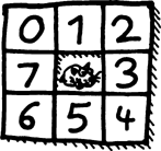
For example, an orientation of 0 would cause the animal to move up and to the left by the next day.
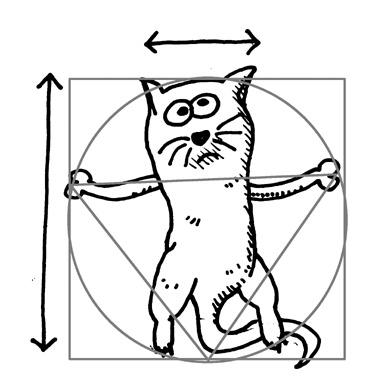
Finally, we need to track the animal’s genes. Each animal has exactly eight genes, consisting of positive integers. These integers represent eight “slots,” which encircle the animal as follows:
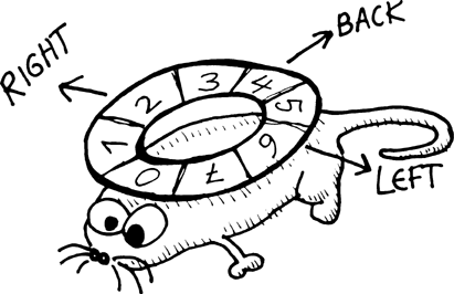
Every day, an animal will decide whether to continue facing the same direction as the day before or to turn and face a new direction. It will do this by consulting these eight slots and randomly choosing a new direction. The chance of a gene being chosen will be proportional to the number stored in the gene slot.
For example, an animal might have the following genes:
(1 1 10 1 1 1 1 1)
Let’s represent these genes as a table, showing each slot number and how large of a value is stored in it:
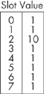
In this example, an animal has a large number (10) stored in slot 2. Looking at our picture of the eight slots around the animal, you can see that slot 2 points to the right. Therefore, this animal will make a lot of right-hand turns and run in a circle. Of course, since the other slots still contain values larger than zero, the animal will occasionally move in another direction.
Let’s create an *animals* variable, populated with a single starting animal. You can think of this animal as “Adam” (or “Eve”, depending on what gender you prefer for our asexual animals).
(defparameter *animals*
    (list (make-animal :x      (ash *width*  −1)
                       :y      (ash *height* −1)
                       :energy 1000
                       :dir    0
                       :genes  (loop repeat 8
                                     collecting (1+ (random 10))))))
We make the animal’s starting point the center of the world by setting the x and y positions to half of the map’s width and height, respectively. We set its initial energy to 1000, since it hasn’t evolved much yet and we want it to have a fighting chance at survival. It starts off facing the upper left, with its dir field set to 0. For its genes, we just use random numbers.
Note that unlike the *plants* structure, which was a hash table, the *animals* structure is just a plain list (currently containing only a single member). This is because, for the core of our simulation, we never need to search our list of animals. Instead, we’ll just be traversing *animals* once every simulated day, to let our critters do their daily activities. Lists already support efficient linear traversals, so using another, more complex data structure (such as a table) would have no significant effect on the performance of our simulation.
The move function accepts an animal as an argument and moves it, orthogonally or diagonally, based on the direction grid we have described:
(defun move (animal)
(let ((dir (animal-dir animal))
(x (animal-x animal))
(y (animal-y animal)))
(setf (animal-x animal) (mod (+ x
(cond ((and (>= dir 2) (< dir 5)) 1)
 ((or (= dir 1) (= dir 5)) 0)
 (t −1))
*width*)
*width*))
(t −1))
*width*)
*width*))
 (setf (animal-y animal) (mod (+ y
(cond ((and (>= dir 0) (< dir 3)) −1)
((and (>= dir 4) (< dir 7)) 1)
(t 0))
*height*)
*height*))
(decf (animal-energy animal))))
(setf (animal-y animal) (mod (+ y
(cond ((and (>= dir 0) (< dir 3)) −1)
((and (>= dir 4) (< dir 7)) 1)
(t 0))
*height*)
*height*))
(decf (animal-energy animal))))The move function modifies the x and y fields, using the animal-x and animal-y accessors. As we’ve discussed, these are automatically generated through the defstruct macro, based on the field names. At the top of this function, we use the accessors to retrieve the x- and y-coordinates for the animal ![]()
![]() . Then we use the same accessors to set the same values, with the aid of
. Then we use the same accessors to set the same values, with the aid of setf ![]()
![]() .
.
To calculate the new x-coordinate, we use a cond command to first check if the direction is 2, 3, or 4 ![]() . These are the directions the animal may face that point east in the world, so we want to add one to the x-coordinate. If the direction instead is 1 or 5, it means the animal is facing directly north or south
. These are the directions the animal may face that point east in the world, so we want to add one to the x-coordinate. If the direction instead is 1 or 5, it means the animal is facing directly north or south ![]() . In those cases, the x-coordinate shouldn’t be changed. In all other cases, the animal is facing west and we need to subtract one
. In those cases, the x-coordinate shouldn’t be changed. In all other cases, the animal is facing west and we need to subtract one ![]() . The y-coordinate is adjusted in an analogous way
. The y-coordinate is adjusted in an analogous way ![]() .
.
Since the world needs to wrap around at the edges, we do some extra math using the mod (remainder) function to calculate the modulus of the coordinates and enable wrapping across the map ![]()
![]() . If an animal would have ended up with an x-coordinate of
. If an animal would have ended up with an x-coordinate of *width*, the mod function puts it back to zero, and it does the same for the y-coordinate and *height*. So, for example, if our function makes the animal move east until x equals 100, this will mean that (mod 100 *width*) equals zero, and the animal will have wrapped around back to the far west side of the game world.
The final thing the move function needs to do is decrease the amount of energy the animal possesses by one. Motion, after all, requires energy.
Next, we’ll write the turn function. This function will use the animal’s genes to decide if and how much it will turn on a given day.
(defun turn (animal)
This function needs to make sure that the amount the animal turns is proportional to the gene number in the given slot. It does this by first summing the amount of all genes, and then picking a random number within that sum ![]() . After that, it uses a recursive function named
. After that, it uses a recursive function named angle ![]() , which traverses the genes and finds the gene that corresponds to the chosen number, based on the respective contributions of each gene to the sum. It subtracts the running count in the argument
, which traverses the genes and finds the gene that corresponds to the chosen number, based on the respective contributions of each gene to the sum. It subtracts the running count in the argument x from the number stored at the current gene ![]() . If the running count has hit or exceeded zero, the function has reached the chosen number and stops recursing
. If the running count has hit or exceeded zero, the function has reached the chosen number and stops recursing ![]() . Finally, it adds the amount of turning to the current direction and, if needed, wraps the number around back to zero, once again by using
. Finally, it adds the amount of turning to the current direction and, if needed, wraps the number around back to zero, once again by using mod ![]() .
.

Eating is a simple process. We just need to check if there’s a plant at the animal’s current location, and if there is, consume it:
(defun eat (animal)
  (let ((pos (cons (animal-x animal) (animal-y animal))))
    (when (gethash pos *plants*)
      (incf (animal-energy animal) *plant-energy*)
      (remhash pos *plants*))))
The animal’s energy is increased by the amount of energy that was being stored by the plant. We then remove the plant from the world using the remhash function.

Reproduction is usually the most interesting part in any animal simulation. We’ll keep things simple by having our animals reproduce asexually, but it should still be interesting, because errors will creep into their genes as they get copied, causing mutations.
(defparameter *reproduction-energy* 200)

  (defun reproduce (animal)
    (let ((e (animal-energy animal)))
     (when (>= e *reproduction-energy*)
       (setf (animal-energy animal) (ash e −1))
       (let ((animal-nu (copy-structure animal))
             (genes     (copy-list (animal-genes animal)))
              (mutation  (random 8)))
          (setf (nth mutation genes) (max 1 (+ (nth mutation genes) (random 3) −1)))
          (setf (animal-genes animal-nu) genes)
          (push animal-nu *animals*)))))
It takes a healthy parent to produce healthy offspring, so our animals will reproduce only if they have at least 200 days’ worth of energy ![]() . We use the global constant
. We use the global constant *reproduction-energy* to decide what this cutoff number should be. If the animal decides to reproduce, it will lose half its energy to its child ![]() .
.
To create the new animal, we simply copy the structure of the parent with the copy-structure function ![]() . We need to be careful though, since
. We need to be careful though, since copy-structure performs only a shallow copy of a structure. This means that if there are any fields in the structure that contain values that are more complicated than just numbers or symbols, the values in those fields will be shared with the parent. An animal’s genes, which are stored in a list, represent the only such complex value in our animal structures. If we aren’t careful, mutations in the genes of an animal would simultaneously affect all its parents and children. In order to avoid this, we need to create an explicit copy of our gene list using the copy-list function ![]() .
.
Here is an example that shows what horrible things could happen if we just relied on the shallow copy from the copy-structure function:
>(defparameter *parent* (make-animal :x 0:y 0:energy 0:dir 0:genes '(1 1 1 1 1 1 1 1)))*PARENT*(defparameter *child* (copy-structure *parent*))*CHILD*(setf (nth 2 (animal-genes *parent*)) 10)10*parent*#S(ANIMAL :X 0 :Y 0 :ENERGY 0 :DIR 0 :GENES (1 1 10 1 1 1 1 1))*child*#S(ANIMAL :X 0 :Y 0 :ENERGY 0 :DIR 0 :GENES (1 1 10 1 1 1 1 1))
Here, we’ve created a parent animal with all its genes set to 1 ![]() . Next, we use
. Next, we use copy-structure to create a child ![]() . Then we set the third (second counting from zero) gene equal to
. Then we set the third (second counting from zero) gene equal to 10 ![]() . Our parent now looks correct
. Our parent now looks correct ![]() . Unfortunately, since we neglected to use
. Unfortunately, since we neglected to use copy-list to create a separate list of genes for the child, the child genes were also changed ![]() when the parent mutated. Any time you have data structures that go beyond simple atomic symbols or numbers, you need to be very careful when using
when the parent mutated. Any time you have data structures that go beyond simple atomic symbols or numbers, you need to be very careful when using setf so that these kinds of bugs don’t creep into your code. In future chapters (especially Chapter 14), you’ll learn how to avoid these issues by not using functions that mutate data directly, in the manner that setf does.
To mutate an animal in our reproduce function, we randomly pick one of its eight genes and place it in the mutation variable. Then we use setf to twiddle that value a bit, again using a random number. We did this twiddling on the following line:
(setf (nth mutation genes) (max 1 (+ (nth mutation genes) (random 3) −1)))
In this line, we’re slightly changing a random slot in the gene list. The number of the slot is stored in the local variable mutation. We add a random number less than three to the value in this slot, and then subtract one from the total. This means the gene value will change plus or minus one, or stay the same. Since we don’t want a gene value to be smaller than one, we use the max function to make sure it is at least one.
We then use push to insert this new critter into our global *animal* list, which adds it to the simulation.
Now that we have functions that handle every detail of an animal’s routine, let’s write one that simulates a day in our world.
(defun update-world ()
First, this function removes all dead animals from the world ![]() . (An animal is dead if its energy is less than or equal to zero.) Next, it maps across the list, handling each of the animal’s possible daily activities: turning, moving, eating, and reproducing
. (An animal is dead if its energy is less than or equal to zero.) Next, it maps across the list, handling each of the animal’s possible daily activities: turning, moving, eating, and reproducing ![]() . Since all these functions have side effects (they modify the individual animal structures directly, using
. Since all these functions have side effects (they modify the individual animal structures directly, using setf), we use the mapc function, which does not waste time generating a result list from the mapping process.
Finally, we call the add-plants function ![]() , which adds two new plants to the world every day (one in the jungle and one in the steppe). Since there are always new plants growing on the landscape, our simulated world should eventually reach an equilibrium, allowing a reasonably large population of animals to survive throughout the spans of time we simulate.
, which adds two new plants to the world every day (one in the jungle and one in the steppe). Since there are always new plants growing on the landscape, our simulated world should eventually reach an equilibrium, allowing a reasonably large population of animals to survive throughout the spans of time we simulate.
A simulated world isn’t any fun unless we can actually see our critters running around, searching for food, reproducing, and dying. The draw-world function handles this by using the *animals* and *plants* data structures to draw a snapshot of the current world to the REPL.
(defun draw-world ()
First, the function uses a loop to iterate through each of the world’s rows ![]() . Every row starts with a new line (created with
. Every row starts with a new line (created with fresh-line) followed by a vertical bar, which shows us where the left edge of the world is. Next, we iterate across the columns of the current row ![]() , checking for an animal at every location. We perform this check using the
, checking for an animal at every location. We perform this check using the some function ![]() , which lets us determine if at least one item in a list obeys a certain condition. In this case, the condition we’re checking is whether there’s an animal at the current x- and y-coordinates. If so, we draw the letter
, which lets us determine if at least one item in a list obeys a certain condition. In this case, the condition we’re checking is whether there’s an animal at the current x- and y-coordinates. If so, we draw the letter M at that spot ![]() . (The capital letter
. (The capital letter M looks a little like an animal, if you use your imagination.)
Otherwise, we check for a plant, which we’ll indicate with an asterisk (*) character ![]() . And if there isn’t a plant or an animal, we draw a space character
. And if there isn’t a plant or an animal, we draw a space character ![]() . Lastly, we draw another vertical bar to cap off the end of each line
. Lastly, we draw another vertical bar to cap off the end of each line ![]() .
.
Notice that in this function, we need to search through our entire *animals* list, which will cause a performance penalty. However, draw-world is not a core routine in our simulation. As you’ll see shortly, the user interface for our game will allow us to run thousands of days of the simulation at a time, without drawing the world to the screen until the end. Since there’s no need to draw the screen on every single day when we do this, the performance of draw-world has no impact on the overall performance of the simulation.
Finally, we’ll create a user interface function for our simulation, called evolution.
(defun evolution ()
First, this function draws the world in the REPL ![]() . Then it waits for the user to enter a command at the REPL using
. Then it waits for the user to enter a command at the REPL using read-line ![]() . If the user enters
. If the user enters quit, the simulation ends ![]() . Otherwise, it will attempt to parse the user’s command using
. Otherwise, it will attempt to parse the user’s command using parse-integer ![]() . We set
. We set :junk-allowed to true for parse-integer, which lets the interface accept a string even if it isn’t a valid integer.
If the user enters a valid integer n, the program will run the simulation for n simulated days, using a loop ![]() . It will also print a dot to the screen for every 1000 days, so the user can see that the computer hasn’t frozen while running the simulation.
. It will also print a dot to the screen for every 1000 days, so the user can see that the computer hasn’t frozen while running the simulation.
If the input isn’t a valid integer, we run update-world to simulate one more day. Since read-line allows for an empty value, the user can just tap the enter key and watch the animals move around their world.
Finally, the evolution function recursively calls itself to redraw the world and await more user input ![]() . Our simulation is now complete.
. Our simulation is now complete.
To start the simulation, execute evolution as follows:
> (evolution)
|
                                             |
|
                                                     |
|
                                                |
|
                                                     |
|
                                             |
|
                                             |
|
                                            |
|
                                     |
|
                                        |
|
                                             |
|
                                        |
|
                                           |
|
                                      |
|
                                      |
|
                                      |
|                                                  M
                                            |
|
                                        |
|
                                             |
|
                                          |
|
                                             |
|
                                      |
|
                                                  |
|
                                         |
|
                                           |
|
                                           |
|
                                              |
|
                                              |
|
                                          |
|
                                           |
|
                                   |
Our world is currently empty, except for the Adam/Eve animal in the center. Hit enter a few times to cycle through a few days:
|
|
|
|
|
|
|
|
|
|
|
|
|
|
|
|
|
|
|
|
|
|
|
|
|
|
|
|
| *
|
|
|
| * M
|
|
|
|
|
|
|
|
|
|
|
|
|
|
|
|
|
|
|
|
|
|
|
|
|
|
|
[enter]Our under-evolved animal is stumbling around randomly, and a few plants are starting to grow.
Next, enter 100 to see what the world looks like after 100 days:
100
|                                                    *
               *                       |
|
           *                       *          |
|  *                 **                            *
                                           |
|           *    *    *
          * *                        |
|                                          M        *
      M*                           *        |
|          *                        M    *
                                       |
|             *           *                                        *
                                 |
|                                        *     M             M *
                                    |
|                                           M M  M
              *                  |
|                       *                        M M             *    *
                              |
|                        *                       M M  MM                *
    *                      |
|                                            M* *
                              *              |
|                                                 M  M    M
          *                         |
|                          *                  M       MM
                                           |
|          *                  *     *      M  M   *      M
   M  *                     *   *          |
|     *                           *    *       M MM   *  M
       *                *               |
|                                            M M   M*  *
         *              *           |
|                        *      *        M    M  M
                                           |
|                   *                                 *    M
                  *              *  *   |
|
   M                               *       |
|         *                           * M               M
                                            |
|   *                 *               *             M     M
                                         |
| *    *                                  *     M M    M
   M                                        |
|               *                         *      M    M
           * *          *                  |
|                                            *
                                   *       |
|                        *             *
          *                            |
|                            *
                       *              |
|        *      *                                 M
                                        *     |
|                        *
                                     *       |
| *                   *                          M              *
           * * *                   |
Our animal has already multiplied quite a bit, although this has less to do with the amount of food it has eaten than with the large amount of “starter energy” we gave it.
Now let’s go all out and run the simulation for five million days! Since we’re using CLISP, this will be kind of slow, and you may want to start it up in the evening and let it run overnight. With a higher-performance Lisp, such as SBCL, it could take only a couple of minutes.
5000000
|                                                                *
      M              M        |
|         *            *          *
                          M               |
|      M
                       *              |
|           M                                       *
       *       M        M                |
|                *                            M            *
        *                             |
|                                                           **
                                  *   |
|                                                M
                                          |
|           M        *                                M              M
       *                       |
|              *                       *     M   M M     M
              M                     M      |
|                                                M
                        M                  |
| M*                                    *     M  M  MMM    M
                                   M     |
|    *              *                     MMM  *           M             M
                       M  |
|  *            M    *               M      M *MM*     MMM M
                           *            |
|                                              M  MMMMMM M M
      M                        *         |
|               M                          MMMM MMM  M *          M
                              M   |
|         M                              *          M MMM
     *                               *   |
|                                             M M M  M M M
     M                           *    |
|      M                                M M  MMM               M
      M       M                 |
|                      M                  M  M    MM
   M             *          *      |
|                                     *     MMM M
 MM M                                        M   |
|                        M                            MM     *
            M                          |
|                                             MMM  M  M   M
                                         |
|           *               M                           M
                                         |
|               M            M          M        *M                *
       M   M                     |
|      M        M
      MM            M                |
|  M                             *                 M   *    M
    M                                 |
|               MM      M      M      M
     M                        |
|                   M       M         M
                                         |
|        M           *    M                    *            *
                *                  |
|        M     M                                     M
                                          |
Our world doesn’t look much different after five million days than it did after a hundred days. Of course, there are more animals, both traveling across the steppes and enjoying the lush vegetation of the jungle.
But appearances are deceptive. These animals are distinctly different from their early ancestors. If you observe them closely (by tapping enter), you’ll see that some of the creatures move in straight lines and others just jitter around in a small area, never taking more than a single step in any direction. (As an exercise, you could tweak the code to use different letters for each animal, in order to make their motion even easier to observe.) You can see this contrast even more clearly by typing quit to exit the simulation, then checking the contents of the *animals* variable at the REPL:
>*animals*
#S(ANIMAL :X 6 :Y 24 :ENERGY 65 :DIR 3 :GENES (67 35 13 14 1 3 11 74))
 #S(ANIMAL :X 72 :Y 11 :ENERGY 78 :DIR 6 :GENES (68 36 13 12 2 4 11 72))
 #S(ANIMAL :X 16 :Y 26 :ENERGY 78 :DIR 0 :GENES (71 36 9 16 1 6 5 77))
 #S(ANIMAL :X 50 :Y 25 :ENERGY 76 :DIR 4 :GENES (2 2 7 5 21 208 33 9))
 #S(ANIMAL :X 53 :Y 13 :ENERGY 34 :DIR 4 :GENES (1 2 8 5 21 208 33 8))
 #S(ANIMAL :X 58 :Y 10 :ENERGY 66 :DIR 6 :GENES (5 2 7 2 22 206 29 3))
 #S(ANIMAL :X 74 :Y 3 :ENERGY 77 :DIR 0 :GENES (68 35 11 12 1 3 11 74))
 #S(ANIMAL :X 47 :Y 19 :ENERGY 47 :DIR 2 :GENES (5 1 8 4 21 207 30 3))
 #S(ANIMAL :X 27 :Y 22 :ENERGY 121 :DIR 1 :GENES (69 36 11 12 1 2 11 74))
 #S(ANIMAL :X 96 :Y 14 :ENERGY 78 :DIR 5 :GENES (71 37 9 17 2 5 5 77))
 #S(ANIMAL :X 44 :Y 19 :ENERGY 28 :DIR 1 :GENES (1 3 7 5 22 208 34 8))
 #S(ANIMAL :X 55 :Y 22 :ENERGY 18 :DIR 7 :GENES (1 3 8 5 22 208 34 7))
 #S(ANIMAL :X 52 :Y 10 :ENERGY 63 :DIR 0 :GENES (1 2 7 5 23 208 34 7))
 #S(ANIMAL :X 49 :Y 14 :ENERGY 104 :DIR 4 :GENES (4 1 9 2 22 203 28 1))
 #S(ANIMAL :X 39 :Y 23 :ENERGY 62 :DIR 7 :GENES (70 37 9 15 2 6 5 77))
 #S(ANIMAL :X 97 :Y 11 :ENERGY 48 :DIR 0 :GENES (69 36 13 12 2 5 12 72))
 ...
If you look closely at all the animals in the list, you’ll notice that they have two distinct types of genomes. One group of animals has a high number toward the front of the list, which causes them to move mostly in a straight line. The other group has a large number toward the back of the list, which causes them to jitter about within a small area. There are no animals with a genome between those two extremes. Have we evolved two different species?
If you were to create a function that measured how far these evolved animals travel in a fixed amount of time, the histogram of the distance would appear as follows:
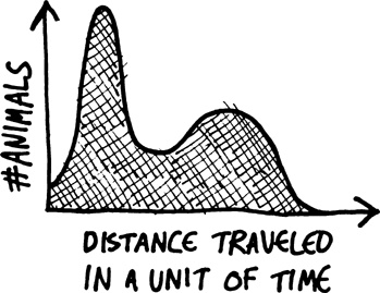
This is a clear bimodal distribution, showing that the behavior of these animals appears to fall into two populations. Think about the environment these animals live in, and try to reason why this bimodal distribution would evolve. We will discuss the solution to this conundrum next.
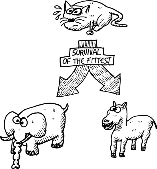
The solution to the evolution puzzle is pretty straightforward. There are two possible survival strategies an animal can adopt in this imaginary world:
Focus on the rich food supply in the jungle. Any animal adopting this strategy needs to be conservative in its motion. It can’t stray too far over time, or it might fall out of the jungle. Of course, these types of animals do need to evolve at least a bit of jittery motion, or they will never find any food at all. Let’s call these conservative, jittery, jungle-dwelling animals the elephant species.
Forage the sparse vegetation of the steppes. Here, the most critical trait for survival is to cover large distances. Such an animal needs to be open-minded, and must constantly migrate to new areas of the map to find food. (It can’t travel in too straight a line however, or it may end up competing for resources with its own offspring.) This strategy requires a bit of naïve optimism, and can at times lead to doom. Let’s call these liberally minded, risk-taking animals the donkey species.
Expanding the simulation to evolve the three branches of government is left as an exercise to the reader.