So far, you have learned that ArcGIS Pro has some powerful tools for visualizing and maintaining GIS data. But what about analyzing that information?Can it help you identify the landowners you need to contact along a road that will be repaired or get a count of customers within a given area? ArcGIS Pro has the tools to help you answer these types of questions and a whole lot more.
Answering these types of questions is done by using geoprocessing tools within ArcGIS Pro. What is Geoprocessing? Simply put, it is the manipulation of data used inside ArcGIS. Geoprocessing tools can analyze data, convert data from one format into another, add an attribute field to a table, or project data from one coordinate system to another. The sky is the limit regarding what you can do with geoprocessing tools.
In addition to the tools included in ArcGIS Pro, you can purchase extensions that add more capability to the software. The geoprocessing framework also provides avenues for you to create your own custom tools using ModelBuilder, Python, and other programming languages. You will learn more about ModelBuilder and Python in later chapters.
In this chapter, you will learn how to use some of the most commonly used geoprocessing analysis tools to perform simple Geographical Information System (GIS) analysis of spatial and tabular data. In addition, you will learn how you can determine which tools will be available to you based on the licensing level and extensions that are assigned to you. As you work through this chapter, you will learn about the following topics:
- Determining which tools to use
- Understanding the analysis process
- Using other common geoprocessing tools for analysis
One thing to keep in mind as you begin to use geoprocessing tools is that most of them create new data. This means that even if you choose the wrong tool or use a bad setting in the tool, in most cases, your original data is protected. This provides a level of protection and helps to put your mind at ease knowing the chances of damaging your data by doing the wrong thing are greatly decreased.
Technical requirements
You must have at least ArcGIS Pro 2.6 or later in order to complete the exercises in this chapter. A Basic, Standard, or Advanced license level will work.
Determining which tools to use
There are two things that determine which geoprocessing tools will be available to you in ArcGIS Pro. The first is your licensing level. The second is what extensions you might have. Let's take a look at these two items and their impact on the geoprocessing tools that will be available for use.
In this section, you will learn how the licensing level that you have impacts the geoprocessing tools that are available to you. You will also learn about some of the extensions for ArcGIS Pro and how they add more analysis capabilities.
Understanding licensing levels
If you remember from Chapter 1, Introducing ArcGIS Pro, ArcGIS Pro has three different licensing levels:
- Basic
- Standard
- Advanced
The license level you have will directly impact the geoprocessing tools you will have access to.
The Basic level is the most limiting license level with the least amount of geoprocessing tools. With this level, you will be able to access simple analysis tools such as Buffer, Union, and Intersect. You will not be able to use tools that allow you to find the closest feature in another layer or that erase overlapping areas between two or more layers.
The Standard level includes a few more geoprocessing tools in addition to all the ones available at the Basic level. Many of these are focused on data management and maintenance. For example, the Standard level includes geoprocessing tools for creating relationship classes within a geodatabase. It also includes tools for managing an Enterprise or Workgroupgeodatabase. Finally, it includes tools for creating and managing topologies that allow you to validate or check your spatial data for errors based on the rules you apply.
The Advanced license level has the greatest amount of geoprocessing tools. It includes all the tools found in the Basic and Standard licenses, in addition to more analysis tools. The Advanced license will allow you to locate the nearest feature to another feature or calculate the distances between points. It also has tools that allow you to erase areas of overlap between two or more layers, plus many more analysis tools.
The following table shows you a comparison of the number of geoprocessing tools found in the Basic and Advanced licensing levels of ArcGIS Pro 2.6. The Standard license level will fall somewhere between the Basic and Advanced licensing levels:
| Parameters | Basic | Advanced |
| Analysis | 19 | 29 |
| Cartography | 11 | 41 |
| Conversion | 36 | 42 |
| Data Management | 210 | 346 |
| Editing | 0 | 17 |
| Geocoding | 11 | 11 |
| Linear Referencing | 7 | 7 |
| Multi-dimension | 11 | 12 |
| Server | 16 | 16 |
| Space-time pattern mining | 9 | 9 |
| Spatial Statistics | 33 | 33 |
| Total | 363 | 563 |
Each licensing level has other limitations besides just which geoprocessing tools are available. You should check Esri's ArcGIS for Desktop Functionality Matrix to see a complete listing of the differences between the licensing levels. ArcGIS Pro will be slightly different as not all the functionality found in ArcGIS for Desktop has been ported into ArcGIS Pro. You can view the functionality matrix by going to https://www.esri.com/content/dam/esrisites/en-us/media/brochures/arcgis-enterprise-functionality-matrix.pdf.
The license level is not the only thing that impacts which tools you can use to perform analysis within ArcGIS Pro. Esri has also created several extensions that provide additional analysis tools.
In the next section, we will briefly discuss the extensions that Esri has currently available for ArcGIS Pro so that you have some idea about what they are and if they might be useful to you.
Learning about extensions for ArcGIS Pro
Esri also has several extensions for ArcGIS Pro that you can purchase. Extensions are add-ons for the core ArcGIS Pro product. They provide extended functionality to all licensing levels. Each extension has a focused area of increased functionality, which includes additional geoprocessing tools.
There are currently 19 different extensions that have been developed for ArcGIS Pro. The current ArcGIS Pro extensions, as of version 2.6, include the following:
- Spatial Analyst
- 3D Analyst
- Network Analyst
- Geostatistical Analyst
- Data Reviewer
- Data Interoperability
- Image Analyst
- Locate XT
- Location Referencing
- Production Mapping
- Publisher
- Workflow Manager
- Maritime Charting
- Defense Mapping
- Aviation Airports
- Aviation Charts
- Bathymetry
- Business Analyst
- StreetMap Premium
The name of each extension helps to identify its purpose. For example, the 3D Analyst extension includes tools you can use to create and analyze data in a 3D environment. The Network Analyst extension allows you to perform analysis across a linear network such as a road network to calculate service areas or determine the shortest travel paths or calculate estimated drive times between two or more points.
To use the previously listed extensions, not only do you need to purchase them, but a license must also be assigned to the user in ArcGIS Online or Portal for ArcGIS. We will take a quick look at the first three extensions – Spatial Analyst, 3D Analyst, and Network Analyst, which are the most commonly used, in the upcoming sections.
Spatial Analyst
The Spatial Analyst extension is used to perform spatial analysis using raster-based data. Things you can do with the Spatial Analyst extension include the following:
- Perform terrain analysis with a Digital Elevation Model (DEM)
- Calculate slopes
- Determine viewsheds
- Perform hydrological analysis
- Classify images and much more
The Spatial Analyst extension includes over 170 geoprocessing tools that can be found in a toolbox with the same name as the extension:
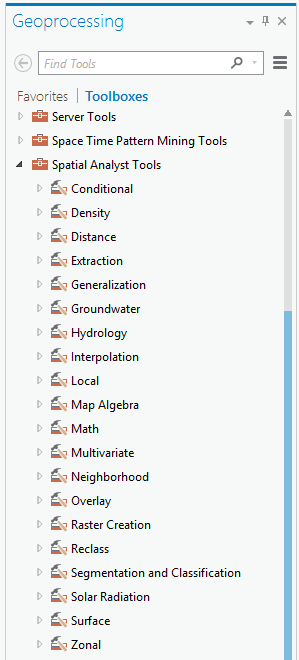
From the preceding screenshot, you can see that these geoprocessing tools are organized into 21 different toolsets within the toolbox.
3D Analyst
The 3D Analyst extension allows you to work with and analyze 3D data within ArcGIS Pro. It has many tools in common with Spatial Analyst. The major difference is that 3D Analyst is designed to work with 3D vector data as opposed to raster data. It does have some ability to create and analyze raster data, but that is not its strong suit. It is not uncommon to use the 3D Analyst and Spatial Analyst extensions together. For example, you might take 3D vector data such as elevation contours and use 3D Analyst to create a DEM for additional analysis with the Spatial Analyst extension.
3D Analyst allows you to work with many 3D datasets, including Triangulated Irregular Networks (TIN), Light Detection And Ranging Laser (LiDAR LAS) datasets, and many of the other standard data formats that were discussed in Chapter 8, Editing Spatial and Tabular Data. If your data does not have an elevation or height associated with it, 3D Analyst can drape your 2D data over a surface and then use that surface to calculate an elevation for your features in relation to the draped surface.
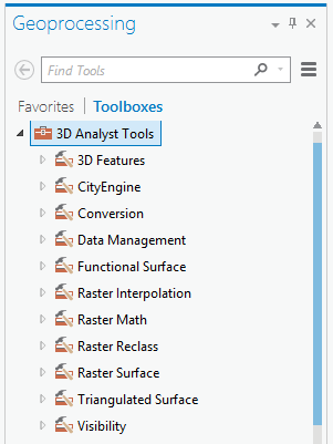
The 3D Analyst extension includes just over 100 geoprocessing tools grouped into 11 toolsets:
As you saw in Chapter 4, Creating 3D Scenes, ArcGIS Pro does support visualizing 3D data as part of its core functionality. So, you might be wondering why you would need the 3D Analyst extension. While visualizing 3D data is part of what ArcGIS Pro allows you to do out of the box with any license level, it does not allow you to perform analysis in 3D. You must have the 3D Analyst extension if you need to determine things such as slope or lines of sight or generate a Digital Elevation Model (DEM) in ArcGIS Pro.
Network Analyst
The Network Analyst extension has tools for creating and analyzing network datasets. A network dataset is a collection of linear features that are connected by nodes that allow for bi-directional flow. This means you can move in either direction along the lines within the network. Network datasets are normally associated with transportation-related networks such as roads, railroads, sidewalks, or bike paths. These are typically not used for utilities as those are normally single-direction flow networks.
With Network Analyst, you can calculate the best routes for vehicles, determine service areas based on drive time requirements, find nearest features within the network, and more. So, you might use this extension to help site a new fire station based on the drive time coverage of existing fire stations.
The Network Analyst extension for ArcGIS Pro currently includes 20 geoprocessing tools organized into three toolsets:

As you can see from the preceding screenshot, the names of the tools should help you understand their purpose and provide a bit more insight into what the Network Analyst extension will allow you to do. For example, the Make Service Area Layer tool will calculate a service area based on a location, along with a Network Dataset. The Build Network tool creates the network dataset that you use as the foundation for the other analysis the extension performs.
Now that you have an understanding of license levels and extensions, the following exercise will show you how to determine which license level and extensions have been assigned to you for ArcGIS Pro so that you can determine what capabilities you have.
Exercise 10A – Determining your license level and extensions
As you have just learned, the license level of ArcGIS Pro and the extensions that you have been assigned will impact what you can do in ArcGIS Pro. So, it is important to know what license level and extensions you have to work with.
In this short exercise, you will determine what license level you have and what extensions (if any) have been assigned from within ArcGIS Pro. If you happen to be the administrator for your organization, you can also log into ArcGIS Online or Portal for ArcGIS to determine what licenses have been assigned to each user. However, not everyone has administrative rights, so it is important to know how you can determine this from ArcGIS Pro.
Step 1 – Opening ArcGIS Pro
The first step is to open ArcGIS Pro and then determine what license level is available to you:
- Open ArcGIS Pro, as you have done in past exercises.
- Click on About ArcGIS Pro, which is located in the lower-left corner of the Open a recent project starting window.
The About ArcGIS Pro window shows you which version of ArcGIS Pro you are using. It also allows you to check whether there are any software updates for ArcGIS Pro.
Step 2 – Determining the license level and extension
Now, you will see what license level you have been assigned and whether any extensions have also been assigned to you:
- Click on Licensing in the left-hand side pane.
- Review what licenses are available to you. This section will tell you which license level is available, while the middle section will tell you what extensions have been assigned to you.
- Close ArcGIS Pro once you have answered the preceding questions.
Now that you know what version of the software you are running, the license level you have been assigned, and if you have any extensions assigned to you, you should have a much better idea of what capabilities are available to you as you work with ArcGIS Pro. With that knowledge of what you have to work with, it is now time to take a look at the analysis process within ArcGIS Pro.
Understanding the analysis process
GIS analysis normally starts with a question. This question can be a simple one such as what the total length of roads within the city is. They can also be very complex, such as I need to know the best place to locate my new business within the city so that it has water and sewer services, as well as whether it is near major roads and in a location that will get business customers during the day and families in the evening.
These questions get you started on the analysis process. This process is normally not linear. You will find that once you answer the initial question, it leads to other questions that start the process all over again. So, the general analysis process looks like this:
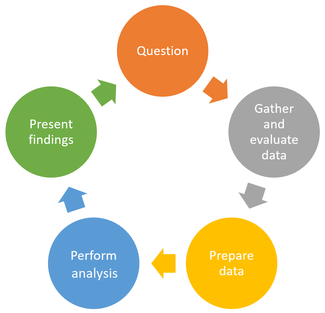
The initial question should cause you to ask questions as well. The question period establishes the specifications of what needs to be answered and what data you will need to answer the question.
Once you know exactly what question you are trying to answer, you need to start gathering the data you will need to perform the analysis. As you gather the data, you need to evaluate it. Does it contain all the information you need?Is it in the format you need?Are the units the correct ones to answer the questions? These are all examples of things you need to consider as you gather the data that you will use for your analysis.
Next, you will need to prepare your data for analysis. This may include simplifying it by clipping it to a specific area, projecting it to a different coordinate system, converting data formats, merging layers, generalizing information, or updating it.
Once you have prepared your data, you are then ready to begin your analysis. This can often require the use of multiple geoprocessing tools, along with other tools such as selecting features based on attributes or locations.
After you have completed your analysis, you will need to present your findings. You can do that by creating a map and layout, as you have already learned. You can also create charts and graphs to display your results.
Preparing data for analysis
As you gather and evaluate data for analysis, it is not unusual for the data to need some preparation work to get it into a state that you can use for your analysis. For example, you may download data from ArcGIS Online that is in a different coordinate system than the primary one you use for your data. So, you would need to project the downloaded data to the coordinate system that you will use for the rest of your data.
Common data preparation tasks include simplifying data, standardizing units, merging layers, and updating the data. Some of the most widely used geoprocessing tools to perform these tasks are as follows:
- Clip
- Dissolve
- Project
- Append
- Merge
These tools are available at all licensing levels. We will learn about each of the aforementioned tools in the following sections.
Clip geoprocessing tool
The Clip tool is used to extract data based on the boundary of other data. For example, if you wanted to determine which portions of streets were located in the city limits, you could use the clip tool to cut out the parts of the streets that are inside the city limits to their own layer. The Clip tool acts like a cookie-cutter.
This tool can be found in the Analysis toolbox and the Extract toolset. It can be used to clip points, lines, or polygons. However, the clipping layer must be a polygon. Here is an example of the Clip tool in action:
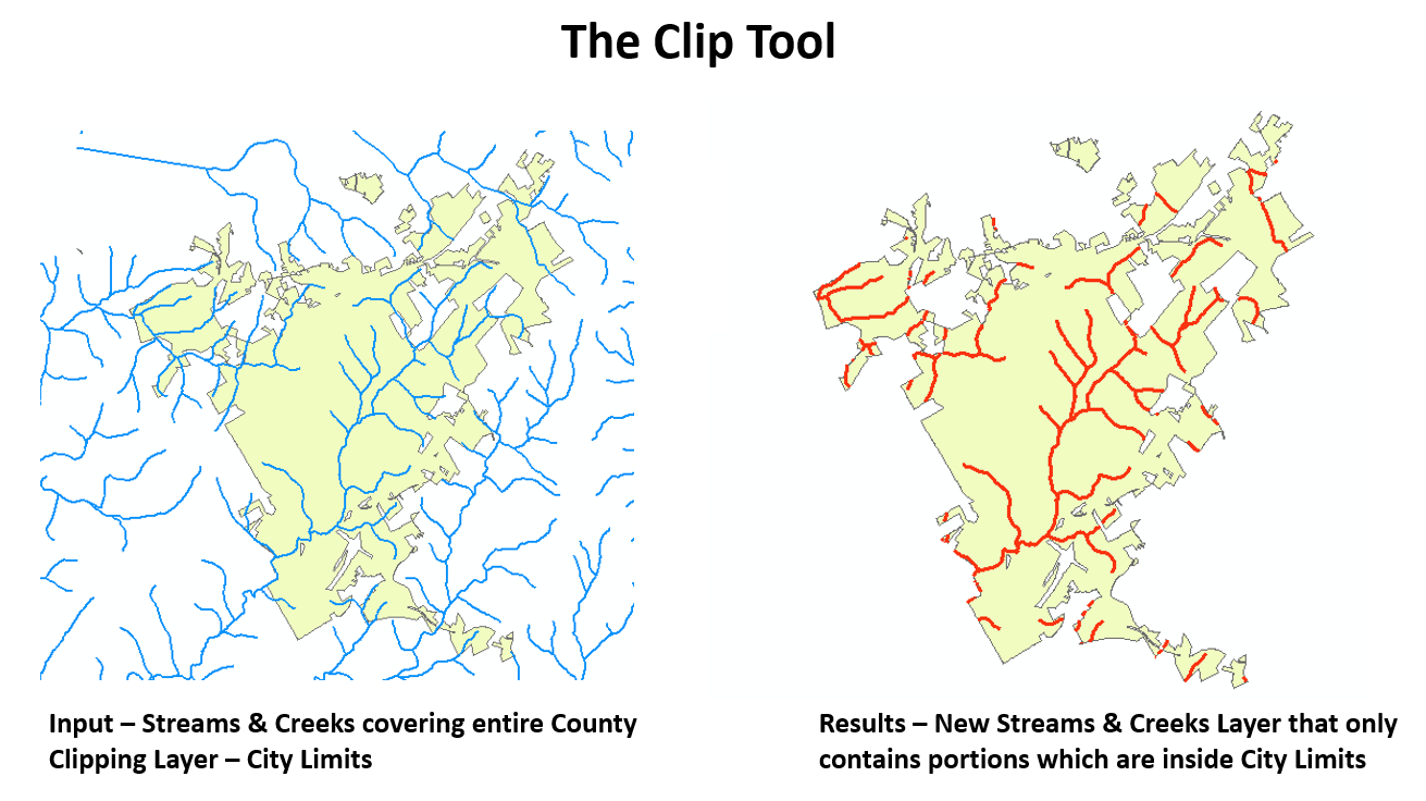
From the previous screenshot, you can see that we are trying to isolate the portions of the creeks and streams that are located inside the city limits. The creek and stream layer contains the location of all of them in the entire county. Here, we have clipped them using the city limits layer, which is a polygon. The result is a new layer that contains only those portions of the streams and creeks that are located inside the city limits.
Dissolve tool
The Dissolve tool is used to simplify or generalize a data layer based on a common attribute value. So, for example, if you had a parcel layer that showed each parcel and each parcel was coded with its designated zoning classification and you wanted to know the total amount of area for each zoning classification within the city, the Dissolve tool can be used to create individual polygons for each zoning classification.
The Dissolve tool can be found in the Data Management Tools toolbox and the Generalization toolset. It works on points, lines, and polygons. Here is an illustration of the example that was described earlier:

As shown in the previous screenshot, the initial parcel layer contained many individual polygons that would have made determining the total area for each zoning classification difficult. Once you use the Dissolve tool, a new layer is created so that each zoning class has a single polygon. From there, it becomes much simpler to determine the total area for each zoning class.
Project tool
The Project tool is used to move a spatial layer from one coordinate system to another. It is important to know that when projecting data between coordinate systems, the actual coordinate values for your features must change. The Project tool will take your existing data and translate it into the new coordinate system using the proper math and translations to create a new layer that is in the designated coordinate system.
The Project tool is located in the Data Management Tools toolbox and the Projections and Transformations toolset. Certain tools and functions work best with different types of coordinate systems. There are two basic types of coordinate systems –Geographic and Projected. If you are trying to measure distances or areas, then a projected coordinate system works best.
Even though ArcGIS Pro will project data on the fly so that even the data that's in different coordinate systems will be displayed together, it is a recommended best practice that you place all the data that you are analyzing into the same common coordinate system. This avoids errors being caused by issues with different units and transformations.
This tool should not be confused with the Define Projection tool, which is located in the same place. The Define Projection tool will assign a coordinate system to a feature class that is undefined. It does not actually project data to a new coordinate system. This is a common mistake for new ArcGIS users.
Merge tool
The Merge tool will take data from two or more layers, or tables, and combine them into a new single output. This is useful if you get the same type of data from multiple sources or locations. For example, let's say you are working with a regional emergency response group and you are trying to develop a regional evacuation plan. You receive road data from multiple jurisdictions. You can use the Merge tool to combine them all into a single layer.
The Merge tool can be found in the Data Management Tools toolbox and General toolset. The Merge tool can be used to combine points, lines, polygons, and even standalone tables. You can only merge similar features, meaning you can only merge points with points, lines with lines, and polygons with polygons.
Here is another example of when you might want to use the Merge tool. You are responsible for inventorying all the fire hydrants within the city. So, you go out over the course of several days collecting the location of these fire hydrants. This results in a layer that shows all the locations you've collected daily. You wish to combine all the collected locations into a single layer:

From the previous screenshot, you can see that the Merge tool creates a new layer that includes all the features and attributes that were originally in the four separate layers. So, now, you have a single layer to manage, update, and analyze.
Append tool
The Append tool is very similar to the Merge tool. It also combines data from multiple layers or tables into one. The big difference between these two tools is that Append is one of the few geoprocessing tools that changes the input data. It will add features or records to the target input.
You might use the Append tool if you have an existing layer of information and you just need to add newly acquired data to it. For example, continuing with the previous hydrant example, after merging the hydrants from the first four days, you collected some data. Now, you go out and collect more hydrant locations. You wish to add those newly collected hydrants to the merged layer to create.
The Append tool would work in this case. It would continue to add the newly collected location to the existing data layer. It would not keep creating new layers that you would need to manage. This is illustrated in the following screenshot:

As shown in the previous screenshot, the hydrants that were in the layer showing the fifth day of the collection have been added to the Hydrant_Merge layer in the results on the right. This illustrates how the Append tool adds data from the input layer to the target layer.
Now that you know about some of the most commonly used geoprocessing tools that are used to prepare data for analysis, it is time for you to get some hands-on experience using them. In the next exercise, you will put what you have learned about the Clip and Dissolve tools into action.
Exercise 10B – Using the Clip and Dissolve tools
The Public Works director is working on a report that he must provide to the City Council to support his budget request. He needs to know the total length of each road within the city of Trippville. He has asked you to provide him with those numbers.
Luckily, you already have the city limit and street data within your geodatabase. However, the street data extends outside the city limits and is broken down into individual road segments. So, you will need to take some time to prepare the data before you can provide him with the numbers that he needs.
Step 1 – Evaluating the data
The director has already provided you with the question and you have verified that you already have the data needed for the project. So, now, you just need to evaluate your data to verify the steps you need to complete the project.
In this step, you will open ArcGIS Pro and review the street and city limit data. You will make sure you have the information you need:
- Start ArcGIS Pro and open the Ex10B.aprx file located in C:StudentIntroArcProChapter10Ex10B.
- Once the project opens, you should see a map with two layers, namely City_Limit and Street_Centerlines. Notice that the streets extend outside the city limits.
- Right-click on the Street_Centerlines layer and select Attribute Table.
- The director wants the total length of each road in the city. Review the table for the Street_Centerlines layer to see whether there is a field that identifies what road each segment belongs to.
- Close the table and save your project.
You have now evaluated your data to determine its suitability to provide the information requested by the director. You know you will have to extract portions of the street centerlines that are located inside the city limits and that you have an identification field you can use to dissolve the street segments by to easily calculate their length.
Step 2 – Clipping the streets
In this step, you will clip the street centerlines, thus creating a new layer that only contains the portions of the streets that are located inside the city limits:
- Select the Analysis tab in the ribbon.
- From the Tools group, which is located in the center of the Analysis tab, select Clip. This should open the Geoprocessing pane on the right-hand side of the interface.
If you do not see the Clip tool, you can use the small arrows located on the right-hand side of the Tools group to reveal more tools.
- Click on the small drop-down arrow located to the right of the cell for Input Features and select the Street_Centerlines layer.
- For the ClipFeatures, select City_Limit using the same process.
- Make sure your OutputFeature Class field is set to C:StudentIntroArcProChapter10Ex10BEx10B.gdbStreet_Centerlines_Clip.
- Leave the XY Tolerance field blank. Your Geoprocessing pane should look like this:

- Once you have verified that you have everything set correctly, click the Run button, which is located at the bottom of the Geoprocessing pane.
This will open the help documentation for the tool. This will provide you with a detailed description of what the tool does, intended use cases, and descriptions of all the parameters. It will also include some sample Python scripting code you can use if you are creating a script that contains the tool you are reviewing. You will learn more about Python in Chapter 12, Automating Processes with ModelBuilder and Python.
When the Clip tool is complete, a new layer will be added to your map named Street_Centerlines_Clip.
- Turn off or remove the Streets_Centerlines layer so that you can see the results of the Clip tool in a better way.
- Right-click on the new layer you just created and select Attribute Table.
- Right-click on the ST_NAME field and choose Sort Ascending. This will sort the records based on the name of each road.
So, now, you can see how the Clip tool created a new layer that only contains those portions of the road that are located inside the city limits. Your original layer remains untouched. You are almost ready to provide the director with the information that he needs. However, you still need to simplify the data so that you can calculate the total length of each road more easily.
Let's move on to the next step regarding simplifying the data.
Step 3 – Simplifying the data and calculating the total length
In this step, you will use the Dissolve tool to simplify the clipped road's centerline layer that you created in the previous step. This will create another new layer in your map:
- Click on the Analysis tab in the ribbon.
- Click on the Toolboxes button in the Geoprocessing group tab. This will reactivate or open the Geoprocessing pane once again.
- At the top of the Geoprocessing pane, select Toolboxes, which is located to the right of Favorites. This will display a list of all the toolboxes included in ArcGIS Pro, in addition to any extensions you have access to.
- Expand the Data Management Tools toolbox.
- Expand the Generalization toolset, which is located in the Data Management Tools toolbox.
- Double-click on the Dissolve tool.
- Set the Input Features field to Street_Centerlines_Clip using the same process that you used for the Clip tool.
- Set the Output Feature Class field to C:StudentIntroArcProChapter10Ex10BEx10B.gdbStreet_Centerlines_Dissolve_Name.
- Set the dissolve field to ST_NAME. The Dissolve tool should now look like this:

- Once you have verified that the Dissolve tool is properly configured, click the Run button.
- A new layer is, once again, added to your map. Right-click on this layer and select Attribute Table.
- Right-click on the ST_NAME field and select Sort Ascending.
- Scroll through the list of records. Pay attention to the number of records associated with each road name.
Now, the information is ready to give to the director. With the dissolve complete, you have a list of each road and its associated total length in the Shape_Length field.
In this step, you used the Dissolve tool to simplify the data so that you could easily provide the director with the values that he has requested. The results of the Dissolve tool have summarized the total length of each road within the city by name. Next, we will move on to the last step that's required to meet the request from the director: exporting the data to an Excel spreadsheet.
Step 4 – Exporting a table to Excel
The director appreciates your efforts. However, he does not have ArcGIS Pro. So, he has asked if you can export your results to an Excel spreadsheet. This will allow him to easily incorporate your results in his report.
In this step, you will export the results of your efforts to an Excel spreadsheet using tools that can be found in the Conversion toolbox:
- Return to the Toolboxes list in the Geoprocessing pane by clicking on the small arrow surrounded by a circle in the upper left-hand corner of the pane.
- Expand the Conversion Tools toolbox and then expand the Excel toolset.
- Select the Table to Excel script tool. This particular tool is actually a Python Script. The scroll icon located next to the tool name identifies it as such.
- Set Input Table to Street_Centerlines_Dissolve_Name.
- Set the output to C:StudentIntroArcProChapter10Ex10BStreet_Lengths_by_Name.xls.
- Verify that your Geoprocessing pane looks as follows and click the Run button:

When the Table to Excel tool is complete, it does not add the resulting Excel spreadsheet to your map. If you wish to view your results, start Microsoft Excel and open the spreadsheet that you just created. It should look very similar to the table you viewed in ArcGIS Pro.
- Close the Geoprocessing pane and save your project.
- Close ArcGIS Pro.
Congratulations! You have just completed your first analysis project using ArcGIS Pro. Next, we will look at some other tools that are commonly used to perform analysis.
Using other common geoprocessing analysis tools
With over 300 geoprocessing tools available, you have only just begun to scratch the surface of the types of analysis that you can perform with ArcGIS Pro. ArcGIS Pro includes tools that allow you to perform spatial analysis of your data as well. This can be broken down into several toolsets including Overlay, Proximity, and Statistics within the Analysis toolbox. We will learn about each of these in the upcoming sections.
Overlay analysis
Overlay analysis compares two or more layers and locating areas where they overlap one another. Depending on which tool you use, you can determine the areas where they overlap, erase the areas where they overlap, or combine the total areas of all the inputs.
The Overlay toolset includes the following tools:
| Tool name | Minimum licensing level | Short description |
| Erase | Advanced | It clips out areas of overlap from input features. |
| Identity | Advanced | It calculates areas of overlap and no overlap. |
| Intersect |
Basic |
It returns only the area of overlap. |
| Union | Basic | It combines a total area of input polygons. |
| Update | Advanced | It replaces the area of overlap with new features. |
| Spatial Join | Basic | It joins attributes from one feature to another based on a spatial relationship. |
| Symmetrical Difference | Advanced | It identifies areas where features do not overlap. |
ArcGIS Pro introduces a new Pairwise toolset, which also performs overlay analysis. The tools in this toolset are designed to be used with extremely large datasets. They will provide similar results to those created with the standard Overlay tools.
Now, we will take a closer look at the two overlay analysis tools that are available at all licensing levels, namely Union and Intersect.
Union
The Union tool takes the input of multiple polygon layers and combines all the information into a single feature class that contains all the data from the input layers (typically two or more). It is important to remember that this tool only works with polygons. It can't be used with points or lines. If you need to perform this type of analysis on points or lines, you will need to use the Identify tool.
You might want to use the Union tool if you wish to determine how much of each parcel was in a floodplain area and how much of each parcel was not in a floodplain area, as shown in the following screenshot:

As you can see, the result is a new layer or feature class that contains the attributes from each part of the floodplain that overlaps part of each parcel and the parts of those two layers that do not overlap. Again, your original inputs are still intact.
Intersect
The Intersect tool takes multiple input layers and returns a new layer that shows where the inputs overlap. The resulting layer attribute table will contain the combined attributes of all the inputs. This tool works with all feature types; that is, points, lines, and polygons. If you input multiple feature types, you get to choose what your resulting output type will be.
You might use the Intersect tool if you are working on an emergency evacuation plan for your community. For example, you might need to determine which roads might be blocked due to flooding, so you need to know which segments are in the floodplain. You can use the Intersect tool to overlay the Street Centerlines with the floodplains to locate where and how much of each road is in the greatest danger of flooding, as shown in the following screenshot:

The resulting output of the Intersect tool in this scenario is a new layer that just contains portions of the streets that are located inside the floodplain area. As with other tools, your original input layers have not been changed in any way.
Let's move on to the next toolset – Proximity.
Proximity analysis
Proximity analysis compares, calculates, or shows distances between features in two or more layers. Proximity tools will generate distance buffers, locate nearest features, or calculate distances between features.
The tools included in the Proximity toolset are as follows:
| Tool name | Minimum license level | Short description |
| Buffer | Basic | It creates polygons around existing features at a set distance. |
| Multiple Ring Buffer | Basic | It can create multiple buffer polygons at various distances. |
| Create Thiessen Polygons | Advanced | It creates polygons around points showing areas of influence. |
| Near | Advanced | It identifies how far the nearest feature is between the input and closest feature layers. |
| Generate Near Table | Advanced | It creates a new standalone table that shows distances between the features in two layers. |
| Polygon Neighbors | Advanced | It identifies what polygons are next to the source polygon, and also calculates other associated information. |
Next, we will take a quick look at the Buffer and Multiple Ring Buffer tools mentioned in the preceding table.
Buffer tool
The Buffer tool is one of the most frequently used tools in ArcGIS. It creates a new polygon layer around the input layer based on a specified distance. The buffer distance can be a single value or can be based on an attribute field in the attribute table of the features being buffered. You can choose to buffer any feature type. You can buffer points, lines, or polygons.
However, the output will always be a polygon, as shown in the following screenshot:

Buffers are extremely useful. They can be used to help determine whether features in one layer are within the distance of another layer. They can also help us create features for other purposes, such as creating the rights-of-way for roads or railroads, as shown in the preceding screenshot.
In this illustration, you can see that a new polygon layer has been created around the existing street centerlines, all at a uniform distance. This new layer represents the rights-of-way for those roads. Also, each new polygon inherits the attribute values of the street that was buffered. This means that the new polygons are attributed to the road name and any other attributes that were linked to the street segments.
One of the options you have when using the Buffer tool is to dissolve the overlapping buffers. If you choose to dissolve overlapping buffers, then any buffers that overlap will be merged into a single polygon. This reduces the number of features that are in the resulting layer. Also, if you choose to dissolve overlapping buffers, the new polygons will not contain the attribute information that was associated with the features that you buffered.
The following screenshot shows the difference between a buffer that has been dissolved and one that hasn't:

As you can see, the Not Dissolved example on the left contains many more polygons than the Dissolved one on the right. The example on the left has many overlapping buffers, so if they are dissolved, they become one.
Multiple Ring Buffer tool
The Multiple Ring Buffer tool is a Python script that runs the Buffer tool multiple times to create concentric buffer rings around the buffered features, as shown in the following screenshot:
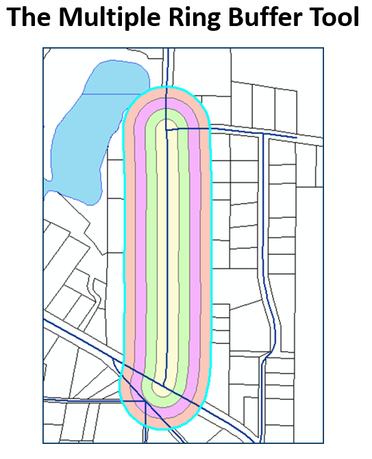
Like the standard Buffer tool, the Multiple Ring Buffer tool works with points, lines, and polygons, but only outputs a new polygon layer. You also have the option to dissolve the overlapping buffers.
Now that you have had an opportunity to learn about some of the most commonly used analysis geoprocessing tools, let's give you a chance to put them into action.
Exercise 10C – Performing analysis
Remember back in Chapter 4, Creating 3D Scenes, when the Community and Economic Development director asked you to prepare several maps that showed the location of commercial properties that were between 1 and 3 acres? After his meeting with the business owners, he needs some more assistance with this project.
He needs you to locate commercial properties that are within 150 feet of existing city sewer lines and that have at least 1 acre that is not in a floodplain.
Step 1 – Locating commercial properties near sewer lines
The first step of your analysis will be to locate all the commercial properties that are between 1 and 3 acres in size and that are within 150 feet of an existing sewer line. Luckily, you identified the commercial properties that meet the size requirements in Chapter 4,Creating 3D Scenes, so that part is done. So, now, you just need to determine which of them are within 150 feet of the sewer lines.
In this step, you will create a 150-foot buffer around the sewer lines in the city. Then, you will perform a spatial selection to select all the commercial properties between 1 and 3 acres that are touched by or intersect with the buffer you create:
- Start ArcGIS Pro.
- Open the Ex10C.aprx project, which is located at C:StudentIntroArcProChapter10.
When the project opens, you should see a map that looks very familiar to the one you created in Chapter 4,Creating 3D Scenes. This map already contains all the basic layers you need to perform your analysis. You can see the commercial properties between 1 and 3 acres, the sewer lines, and the floodplains. Now, you will need to create the 150-foot buffer around the sewer lines.
- Select the Analysis tab in the ribbon.
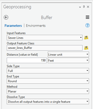
- Select the Buffer tool to open the Geoprocessing pane and Buffer tool parameters.
- Using the skills you learned in the previous exercise, set the Input Feature class to Sewer Lines.
- Set your Output Feature Class to C:StudentIntroArcProChapter10Ex10BEx10B.gdbsewer_lines_Buffer.
- Set the Distance field to 150 and the units to Feet.
- Leave the Side Type, End Type, and Method fields with the default settings.
- Set the Dissolve Type field to Dissolve all output features into a single feature. Since you do not need to know which sewer line is near which parcel, this allows ArcGIS Pro to dissolve the resulting buffer, thus making future analysis easier.
- Verify that your Geoprocessing pane looks as follows and click Run:
Once you've finished using the Buffer tool, a new layer will be added to your map. This new layer will show the areas that are within 150 feet of the sewer lines. You will now use that new layer to select the commercial properties.
- Click on the Map tab in the ribbon.
- Select the Select by Location button in the Selection group on the Map tab.
- The Select by Location tool window will open. Set Input Feature Layer to Commercial Properties 1 to 3 AC.
- Set the Relationship field to Intersect. This will select all the commercial properties between 1 and 3 acres that are overlaid by the sewer lines buffer layer.
- Set the Selecting Features field to sewer_lines_Buffer.
- Leave all the other parameters with their default settings.
- Verify the Select by Location tool window looks as follows and click OK:
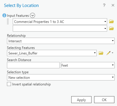
When the Select By Layer Location process completes, you should have approximately 18 commercial properties selected. All of these are overlapping or being touched by the sewer line buffer that you created. This means they are all within 150 feet of an existing sewer line. You will now export those selected parcels to their own layer.
Step 2 – Exporting selected parcels
Now that you have identified which commercial properties are within 150 feet of a sewer line, you will export those to a new feature class so that you can use them for further analysis later. This will ensure you don't mistakenly change or corrupt the existing layer by accident:
- Select Commercial Properties 1 to 3 AC in the Contents pane.
- Select the Data tab in the Feature Layer group.
- Click on the Export Features button located in the Data tab to open the Export Features tool window.
- The Input Features field should automatically be set to Commercial Properties 1 to 3 AC. If not, set it to that layer.
- Set the Output Feature Class field to C:StudentIntroArcProChapter10Ex10Ex10B.gdbCommercialProp_near_sewer.
- Verify that your Export Features window looks as follows and click OK:

When the process for the Copy Features tool completes, a new layer will be added to your map that contains only the commercial parcels that you had selected. If you have features selected in a map or table, most geoprocessing tools will automatically only use those selected records within that tool.
- Open the attribute table for the CommercialProp_near_sewer layer that was just added to your map.
- Verify the table contains the same number of records that you selected previously. There should be approximately 18.
- Clear your selection by clicking on the Clear button in the Selection group on the Map tab.
- Close the table.
- Turn off Sewer Lines, Sanitary Sewer Manholes, sewer_line_Buffer, and Commercial Properties 1 to 3 AC layers. You do not need to see those for the rest of your analysis. They might cause confusion.
- Save your project.
You have just successfully exported the features you had selected to a new feature class, leaving the original data intact. You will use the new feature class you just created in the next step to perform an analysis to determine how much of the commercial properties are located inside the floodplains.
Step 3 – Determining how much of each commercial property is in the floodplain
Now that you have selected the commercial properties that are the required size and that are near the city's sewer system, it is time to calculate how much area of each of those parcels is within the floodplain. To do that, you will use the Union geoprocessing tool to union the new layer that you just created with the floodplains.
This will create a new layer that will split each commercial property into the part that is in the floodplain and the part that isn't:
- Using the skills that you have already learned, open the attribute tables for both the CommercialProp_near_sewer and Floodplains layers. Take a moment to review what fields are located in each table and some of the values that they contain. This will help you understand the results produced by the Union tool.
- Close the tables.
- Click on the Analysis tab in the ribbon.
- Select the Union tool from the Tools group. The Geoprocessing pane will now display the parameters associated with the Union tool.
- Set your input feature classes to Commercial Properties 1 to 3 AC and Floodplains.
- Set your Output Feature Class to C:StudentIntroArcProChapter10Ex10BEx10B.gdbCommercial_Floodplain_Union.
- Once you've verified that your Geoprocessing pane looks as follows, click Run:

When the process for the Union tool completes, it will add a new layer to your map that includes features that are the results of combining the two input layers. Your map should look similar to the following (remember, your colors might be different):

As you can see, the green layer on the map is the result of the Union tool.
- Open the attribute table for the layer that you just created and that was added to your map.
- Select Sort Descending on the SFHA field. All those polygons that are attributed to IN are inside the floodplain. All those that are blank, or NULL, are outside.
- You need to update the ACRE_CALC field to reflect the new acreage for Commercial_Floodplain_Union. Right-click on the ACRE_CALC field and select the CalculateField option.
If the Calculate Field option is grayed out, make sure the layer is editable in the Contents pane on List by Editable. If a layer is not editable, you cannot run the Calculate Field or Calculate Geometry tools.
- Set the Expression Type field to Arcade using the drop-down arrow.
- In the Expression cell located below the Fields column where it says ACRE_CALC =, type $feature.Shape_Area / 43560. This will convert the Shape_Area field values that are in square feet into acres. It should look something like this when you are done entering this value:
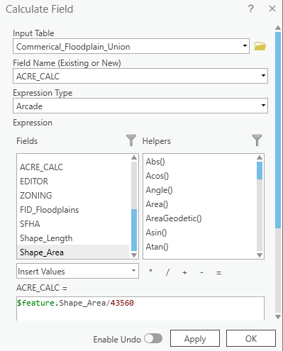
- Click OKonce you have verified your expression.
- Close the table and save your project.
With that, you have used the Union tool to determine how much of each commercial property is within a floodplain and how much is not in the floodplain. Then, you used the Field Calculator tool to calculate the total area of each in acres so that you will be able to complete the next step. In the next step, you will build a query that will select all the commercial properties that are not within a floodplain and are greater than or equal to 1 acre in size.
Step 4 – Selecting commercial parcels that are not in the floodplain
The one problem with using the Union tool in this process is that the resulting layer also includes parts of the floodplain polygons that did not overlap the commercial parcels. This means you need to either simplify that layer by removing those polygons that are in the floodplains or account for them in your query. If you had an Advanced license, you could have used the Identity tool, which would have resulted in you avoiding this step.
In this step, you will select the commercial properties that have at least 1 acre or more not in a floodplain:
- Click on the Map tab in the ribbon.
- Click on the Select by Attributes button to open the tool window.
- Verify that Input Rows is set to Commercial_Floodplain_Union. If not, set it accordingly.
- The Selection type field should be set to New selection.
- Click on the New Expression button.
- After the word Where, set the field to Zoning and the following operator to is not equal to. For the value, select the blank option at the top of the list and click Add. This will eliminate the polygons that just represent floodplain areas that do not overlap the commercial properties.
- Click the Add Clause button located below the clause you just created.
- Set the query field to ACRE_CALC and the following operator to is Greater Than or Equal to. Type in 1.00 for the value and click Add. This selects all the commercial parcels that are of the right size.
- Click the Add Clause button one more time.
- Set the query field to SFHA and the operator to is not equal to. Then, set the value to IN and click Add. This removes any areas that are inside the floodplain from your final selection.
- Click the green checkmark to validate your query. Your Geoprocessing pane should look similar to this:

- Click OK once you've verified everything is set properly. When it is complete, you should have 21 commercial properties selected. These should all be larger than 1 acre in size and outside the floodplain.
- Using the skills you learned about in the previous step, export your selection to a new layer. Set the symbology for the new layer to something that stands out.
- Turn off the Commercial_Floodplain_Union layer so that your new layer stands out even more.
- Save your project.
With that, you have just identified the parcels within the city that meet the director's requirements. You used various analysis and selection tools to answer his question. As you can see, it is not unusual to use multiple tools and methods to get the required answers to what may seem to be a simple question. Believe it or not, once you get familiar and comfortable with these tools, the process you just completed can be done in less than 10 minutes. It just takes practice.
Next, you will learn how to access the history of all the geoprocessing tools you use in ArcGIS Pro.
Step 5 – Reviewing your geoprocessing history
The analysis process you just completed involved many steps. If this was not an exercise with notes to refer to, how would you know all the steps and tools you used to complete the analysis? Luckily, ArcGIS Pro keeps a record of the geoprocessing tools you use, the parameters you included in those tools, and the results or any errors that were encountered. This provides you with a record of the work you did to arrive at your results.
In this step, you will learn how to access this historical record of your geoprocessing activities:
- Click on the Analysis tab in the ribbon.
- Click on the History button, which is located in the Geoprocessing group on the Analysis tab. This will open the History pane.
- Take a moment to review the records you can see in the History pane. You should see all the geoprocessing tools you have used in this chapter listed, as well as any others you might have used in previous chapters or while doing your daily activities.
- Right-click on the Clip tool in the History pane and select the View Details option from the menu. This will look as follows:
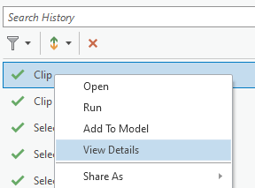
- A new window should open in ArcGIS Pro displaying the history of this instance of the Clip tool when you ran it. Take a moment to review the information contained in this window.
- After you are done reviewing the history of the Clip tool, close the window.
- Right-click on the Clip tool again to display the menu. Review the options it contains.
- Save your project and close ArcGIS Pro.
Now, you know how to access the history of all the geoprocessing tools you use within ArcGIS Pro. This allows you to see the tools you used to complete an analysis, determine what might have caused a tool to fail, and more. You can also rerun the tool from the History pane using the exact same setting that was used at the time shown in the pane. This can help save you time by not having to reenter all the parameters again to run a tool. As you can see, the History pane can be a powerful ally when you need to perform analysis.
Summary
In this chapter, you learned that ArcGIS Pro can be used to conduct spatial analysis to help answer a wealth of questions and concerns. It can also help you see patterns and solutions. You now have the skills to use powerful geoprocessing tools that can be used with various types of data to get the answers you need to everyday problems.
In this chapter, you also learned what geoprocessing is and some of the tools that are available in ArcGIS Pro. You then learned how your licensing level and extensions can impact specific tools that are available to you when you need to perform analysis or manage GIS data.
This chapter also exposed you to some of the most commonly used analysis and data preparation tools. You conducted two separate analysis projects using those tools. With the skills and hands-on experience that you have acquired, you can integrate these tools with other tools that you have already been exposed to in order to find answers.
With that, you have learned many skills, including creating projects, maps, scenes, and layouts using ArcGIS Pro, as well as how to edit and analyze data. You have also seen that there is often more than one way to perform the same task.
In the next chapter, you will explore Tasks, which can allow you to standardize workflows to help train new users, document proper workflows, and ensure everyone is using the same methods to complete common processes.