As you have now learned, performing analysis or editing a feature requires many steps. The more you use ArcGIS Pro, the more you will find yourself doing the same process again and again. You may also realize that some of the processes that you do repeatedly really require very little interaction on your part beyond selecting a feature and then telling ArcGIS Pro where to save the outputs.
Wouldn't it be beneficial if you could automate processes that you perform repeatedly? You can create the proverbial Easy button where you simply click on a single tool, fill in a few parameters, and the tool goes off, providing you with the results after it is done executing. This would certainly make your job easier.
In this chapter, with ArcGIS Pro, you will learn how to create Easy buttons or tools using ModelBuilder and Python scripts. This will provide you with the skills to create automated processes that can run multiple tools together in sequence or at the same time to complete an operation. ModelBuilder uses a visual interface to create automation models without the need to be a programmer.
Python is the primary scripting language for the ArcGIS platform. With it, you can create very powerful scripts that can be used within ArcGIS Pro, but also that can also integrate processes across all components of ArcGIS, includingEnterprise,Online,Extensions,Portal, and more. However, creating Python scripts does require writing code.
In this chapter, you will learn the following topics:
- Differentiating between tasks, geoprocessing models, and Python scripts
- Creating geoprocessing models
- Running a geoprocessing model
- Making a model interactive
- Learning about Python
Technical requirements
As with other chapters in this book, you will need to have ArcGIS Pro 2.5 or later. Any license level of ArcGIS Pro will work for the exercises in this chapter.
Differentiating between tasks, geoprocessing models, and Python scripts
You learned about tasks in the last chapter and have read the introduction for this chapter; now you may be wondering what the difference is between a task, geoprocessing model, and Python script. That is a great question.
You will find the answer to this question in this section, but to understand it, you must first understand what each of these things is. You already know what a task is, so we will now focus on gaining a better understanding of what models and Python scripts are. Once you understand that, you can then understand the differences between the three.
Learning about geoprocessing models
A geoprocessing model is a custom tool created within the ModelBuilder window, which contains multiple geoprocessing tools along with their various parameters (including inputs, outputs, options, and other values) that work together as part of an integrated process that will run as if it was a single tool. The following diagram shows a sample of a very simple model:
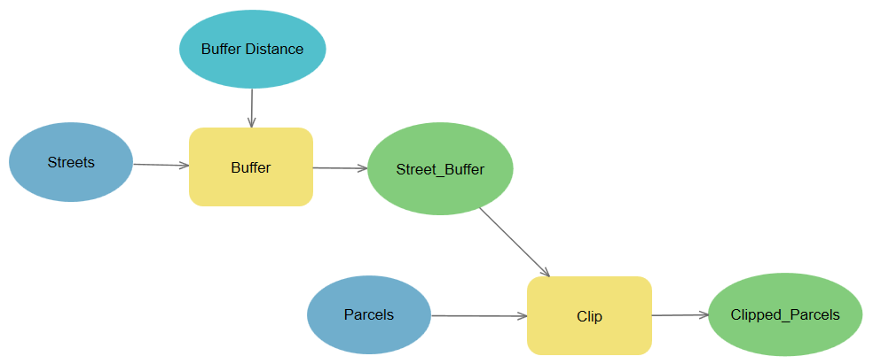
From the preceding diagram, you can see that it contains two geoprocessing tools that you learned about in Chapter 10, Performing Analysis with Geoprocessing Tools, the Buffer and Clip tools. In the model, the Buffer tool creates buffer polygons around the input, Streets.
The resulting buffer polygons are then used to clip out the features in Parcels, which is the Clip features input that is located inside the buffer polygons. Since both geoprocessing tools reside inside the model, the user only has to run the model instead of having to run each tool individually. The model automatically runs the tools based on the parameters specified within it. You will learn more about the components of a model and how to create one later in this chapter.
Geoprocessing models can include geoprocessing tools, Python scripts, iterators, model-only tools, and other models. This allows them to be as simple or complex as you need them to be to accomplish the process that you have designed them to complete. The ModelBuilder window allows users to create geoprocessing models in a visual environment. No coding is required to build a model.
Geoprocessing models can be created using ArcGIS Desktop (ArcMap or ArcCatalog) or ArcGIS Pro. However, models created in one software do not always run successfully in the other. The simpler a model is, the more likely it will be cross-application compatible. Another downside to a geoprocessing model is that it can only be run from ArcGIS Pro or ArcGIS Desktop. You cannot schedule them to run automatically at a specific date and time. At least not by themselves.
Let's now learn about Python scripts.
Understanding Python scripts
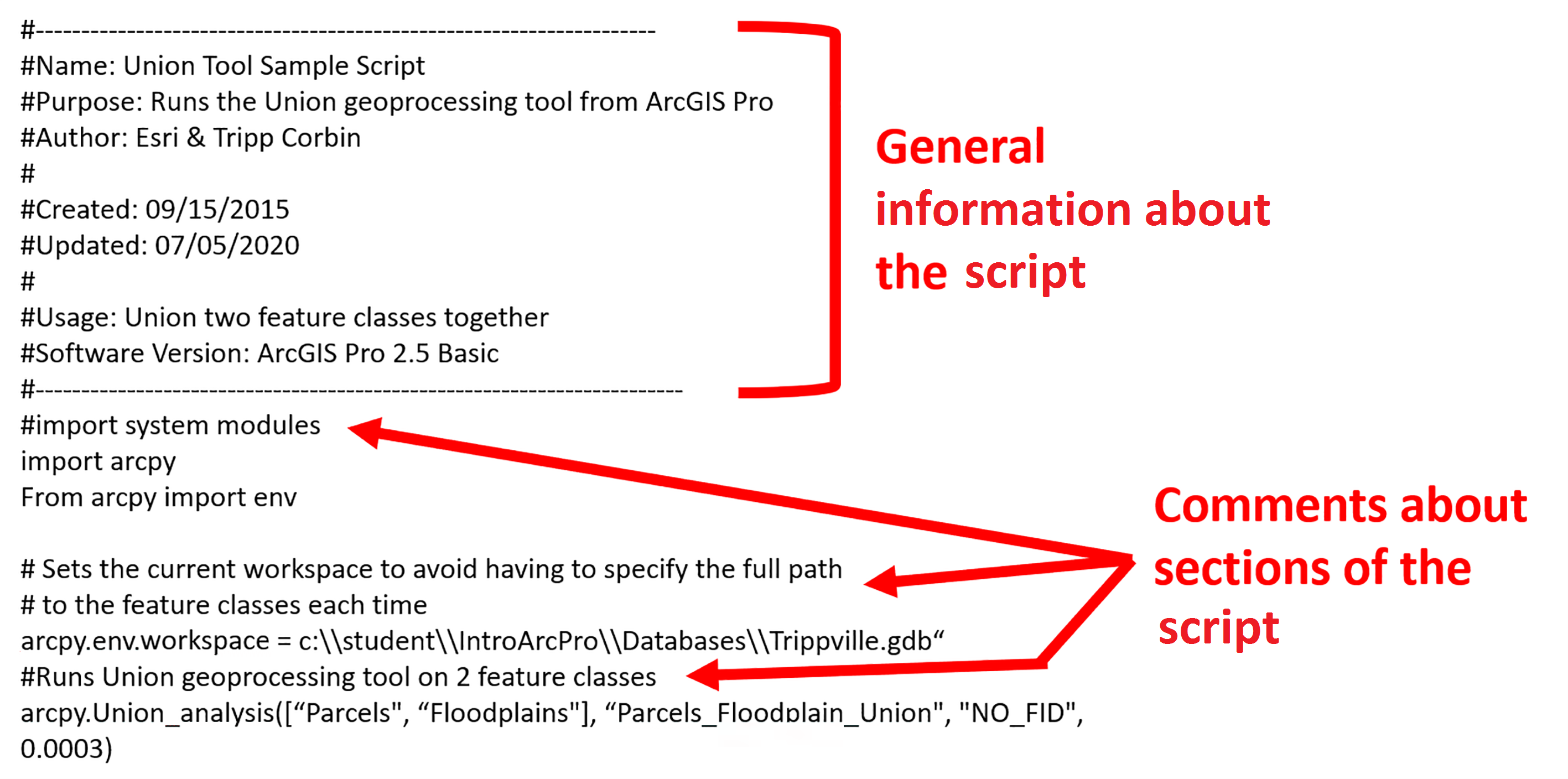
A Python script is also a custom tool that can run multiple geoprocessing tools along with their various parameters as part of an integrated process. However, unlike a model that does not require you to write programming code, Python scripts do. You must know the Python scripting language in order to create Python scripts. The following code is a small snippet of a Python script created for ArcGIS:
#--------------------------------------------------------------
# Name:        Union Tool Sample Script
# Purpose:     Runs the Union Geoprocessing tool from ArcGIS
# Author:      Esri & Tripp Corbin
#
# Created:     09/15/2015
# Updated:     05/08/2020 by Tripp Corbin, GISP
#
# Usage: Union two feature classes
#---------------------------------------------------------------
# Import the system modules
import arcpy

# Sets the current workspace to avoid having to specify the full path
# to the feature classes each time
arcpy.env.workspace = "C:\student\IntroArcPro\Databases\Trippville_GIS.gdb"

#Runs Union Geoprocessing tool on 2 Feature classes
arcpy.Union_analysis (["Parcels", "Floodplains"], "Parcels_Floodplain_Union", "NO_FID", 0.0003)
The preceding code starts with several comment lines that provide a general description of the purpose of the script and who created it. The next line after the commented description is an import command that loads the arcpy model so that the script can access ArcGIS functionality. This is followed by some more descriptive comments, and then a variable is defined to set the workspace where data used in the script will be accessed or saved to. Lastly, the script runs the Union tool, which you learned about in Chapter 10, Performing Analysis with Geoprocessing Tools.
Python scripts have several advantages over a geoprocessing model:
- First, Python is not limited to ArcGIS. Python can actually be used to create scripts for many other applications, such as Excel, SharePoint, AutoCAD, Photoshop, SQL Server, and more. This means that you can use a Python script to run tools across multiple platforms to create a truly integrated process.
- Second, Python scripts can be run from outside of ArcGIS. This means you can schedule them to run at specific times and days using your operating system's scheduler application. If your script does include ArcGIS geoprocessing tools, the script will require access to an ArcGIS license to run successfully, but ArcGIS does not need to be open and active at the time when the script is scheduled to run.
- Third, Python can be used to create completely custom geoprocessing tools. It is not limited to just the geoprocessing tools that you will find in ArcGIS Pro toolboxes.
Now let's see the difference between tasks, geoprocessing tools, and Python scripts.
What is the difference between the three?
Now that you have a much better understanding of what tasks, geoprocessing models, and Python scripts are, you will be able to properly understand the differences between them. Each can serve a purpose in standardizing and automating common workflows and processes.
The following table will provide a clearer understanding of the differences between the three:
| Parameters | Task | Geoprocessing model | Python script |
| Run a single geoprocessing tool automatically | Yes, it can run a single tool automatically as part of a step. | Yes | Yes |
| Allow users to provide input to tools before running | Yes | Yes | Yes |
| Run multiple geoprocessing tasks automatically and in sequence | No | Yes | Yes |
| Be included in a task | No | Yes | Yes |
| Be included in a geoprocessing model | No | Yes | Yes |
| Provides a documented workflow | Yes | Yes | No |
| Run from outside (externally) of ArcGIS Pro | No | No | Yes |
| Integrate with other applications | No | No | Yes |
| Be scheduled to run at specific times and days | No | No | Yes |
| Requires knowledge of programming language | No | No | Yes |
So, as you can now see from the preceding table, there is a good bit of difference between tasks, geoprocessing models, and Python scripts. Tasks are for defining workflows that include several steps. A task might include the use of a geoprocessing model or a Python script, but a geoprocessing model or a Python script cannot reference a task.
Now that you have an understanding of the differences between tasks, geoprocessing models, and Python scripts, we will start exploring how to create a geoprocessing model.
Creating geoprocessing models
As mentioned earlier, geoprocessing models are custom tools that you create from within ModelBuilder. ModelBuilder provides the graphical interface for building models as well as allowing you to access additional model-only tools, iterators, environmental settings, and model properties.
Models are created for several reasons. The first and most common reason is to automate repeated processes performed in ArcGIS Pro. If you have an analysis, a conversion, or another process that you perform on a regular basis, then a model can be used to automate it.
Secondly, you can use a model to think through and create a flow chart process within ArcGIS Pro. This can help you ensure that you have considered all the tools and data that you will need to complete a process. Once completed, the model then provides the tool for completing that process as well as the visual and textual documentation that explains how the process was performed.
You can share models with those in your organization so that they can use it to perform the process. This can reduce your workload and allow you to concentrate on other tasks that require higher knowledge and skill levels. Because a model runs the geoprocessing tools contained within it automatically, you can create a model that is easy for other less Geographic Information System (GIS)-savvy members of your organization to run by themselves without needing a full understanding of ArcGIS Pro. This also helps standardize our methodologies, ensuring that everything is done in a consistent and approved manner.
All of this helps to save us time and money through increased efficiency, which is ultimately the main power of ModelBuilder. Like tasks, models consist of multiple components and have their own terminology associated with them. We will learn about this in the next section.
Understanding model components and terminology
Before you can create a model, you need to understand the pieces and parts that form them. Models include a series of connected processes. Each process includes a tool that can be a geoprocessing tool, another model, or a Python script. Each tool has variables that serve as inputs or outputs.
The following diagram shows you two connected processes:

As you can see in the preceding diagram, the model contains two processes built around the Buffer and Union tools. Each of these tools has a number of variables feeding into it. Variables are identified by the blue and green ovals. Notice that the two processes are sharing a variable – Street_Buffer. This variable is an output of the Buffer tool and also an input for the Union tool.
There are three basic types of variables that are included in a model. They are as follows:
- Data variables: These variables are existing data that is used as an input to a tool, script, or model. These can be layers in a map, standalone tables, text files, feature classes, shapefiles, and more.
- Value variables: These variables are additional information that a tool may use to run. In the case of the Buffer tool, the distance used to create the buffer is considered a value variable as are the options to dissolve, end type, and the other parameters found that appear when you run the Buffer tool normally in the Geoprocessing pane.
- Derived variables: These variables are the outputs of a process. Again, this can be a new layer, feature class, table, raster, or more depending on the tool used in the process.
The following diagram shows you an example of the three types of basic variables in a model:

Since ModelBuilder is a visual programming language, as you can see from the preceding diagram, you can distinguish the types of variables based on their colors. While you can adjust these settings by default, Data Variable is a darker blue. Value Variable is a lighter blue and Derived Variable is green.
Next, we will learn how to save a model that you have created.
Saving a model
If you wish to save a model that you created so that you can use it again or share it with others, you must save it in a custom toolbox that you will create. Models cannot be saved in a system toolbox that is automatically included with ArcGIS Pro when it is installed.
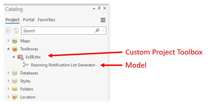
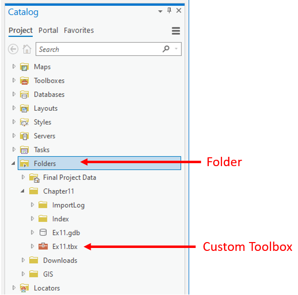
When you create a new project, ArcGIS Pro automatically creates a custom toolbox for that project. It is stored in the Project folder as a .tbx file. This provides you with an easy to use place to store your models. This toolbox is also automatically linked to your project and accessible in the Catalog pane, as follows:
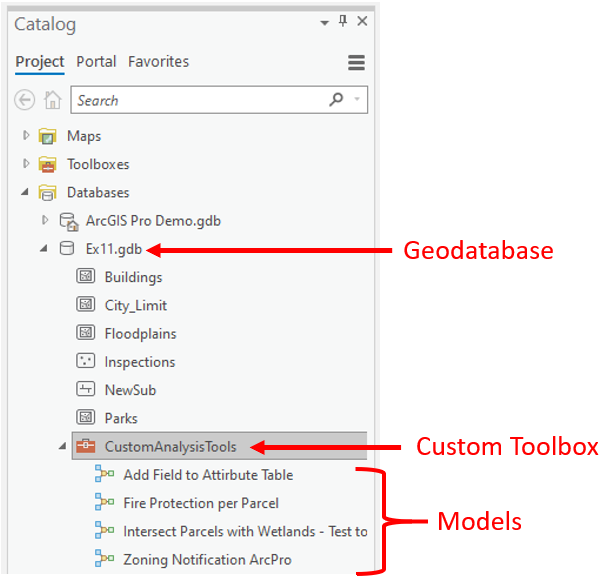
You can also create custom toolboxes within a geodatabase so that along with it, your models and Python scripts are stored as well with your GIS data, as illustrated in the following screenshot (this is a good option if the models or tools that you save to the toolbox will be used in multiple ArcGIS Pro projects):
You can also create other custom .tbx files besides the one that is automatically created with a new project. Using a custom .tbx file is perfect if the tool and models you save to it will not only be used with multiple projects but also across multiple databases or in the case of consultants and multiple clients. The following screenshot shows you an example of a custom toolbox file located in a folder:
Using custom .tbx files to store models also makes it easier to share them with others since they are smaller than a geodatabase, which also includes all the GIS data. The .tbx files can easily be emailed, uploaded to File Transfer Protocol (FTP) sites, or placed in your ArcGIS Online account.
Now that you have a good general understanding of what a model is, its components, and how to save one, it is time to put that knowledge to use.
Exercise 12A – Creating a model
A new ordinance was just passed to protect the streams in the Trippville area. It requires all new building or improvement projects to take place at least 150 feet from the centerline of all creeks or streams. This will hopefully protect the banks from erosion and reduce polluted runoff from reaching them.
The community and economic development director has asked you to calculate the total area of each parcel that is inside the non-disturb area and how much of each parcel is out. Since you will need to update this analysis anytime a new subdivision or commercial development is added, for this, you have decided to create a model that you can run every time you need to perform these calculations.
In this exercise, you will create a simple model that will calculate how much of each parcel is inside and outside a non-disturb buffer area around the streams. This model will include a couple of geoprocessing tools and their associated variables.
Step 1 – Opening the project and the ModelBuilder window
The first step is to open the project and then the ModelBuilder window so that you can begin creating the model:
- Start ArcGIS Pro and open the Ex12.aprx project found in C:StudentIntroArcProChapter12.
- When the project opens, expand the Toolboxes folder in the Catalog pane.
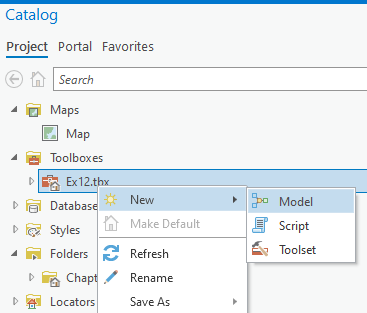
- Right-click on the Ex12 toolbox that you see on your screen.
- Select the New | Model option, as illustrated in the following screenshot:
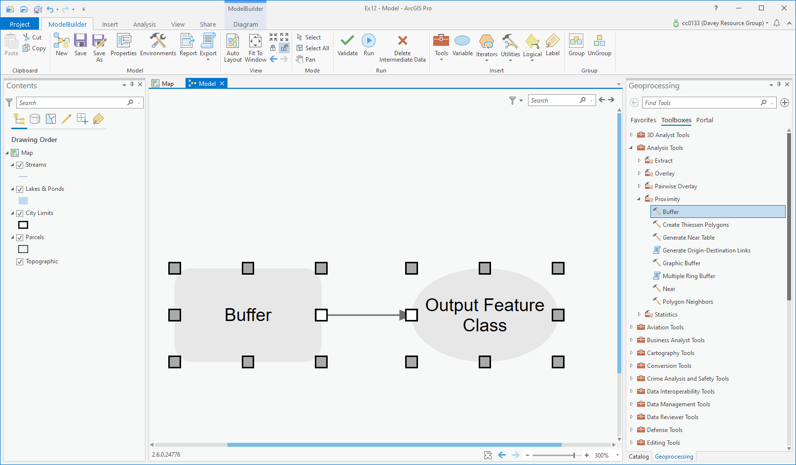
ModelBuilder should now be open and the ModelBuilder tab should have appeared in the ribbon. The ModelBuilder window and tab are used together to create or edit models. As you can see in the following screenshot, the ModelBuilder tab contains tools for saving the model, navigating in the ModelBuilder window, and adding content to the model:

You will now begin using these tools to create your model.
Step 2 – Adding model components
In this step, you will begin adding tools and variables to your model. You will explore some of the different methods that can be used here. You will start by adding the process that will generate the non-disturb buffers around the streams:
- Click on the Tools button on the Insert group on the ModelBuilder tab in the ribbon. This opens the Geoprocessing pane on the right side of the interface.
- Click on the Toolboxes tab at the top of the pane to expose the various toolboxes within ArcGIS Pro. These toolboxes will be your system toolboxes.
- Expand the Analysis Tools toolbox and then the Proximity toolset.
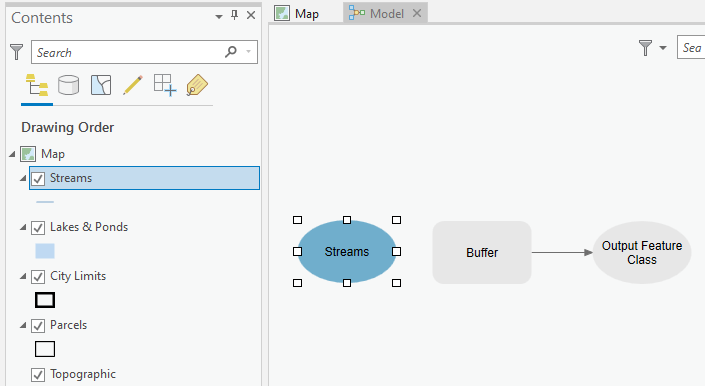
- Drag and drop the Buffer tool from the toolbox into the ModelBuilder window so that it looks like this:
You have just added your first process to a model. Model processes will exist in one of three states: not ready to run, ready to run, and have been run. The process that you just added is in the not ready to run state.
ArcGIS Pro indicates that visually by displaying the tools and variables in gray. A process will be in the not ready to run state until all required variables have been defined. In the case of the Buffer tool, you have not yet defined the three variables required: input feature class, buffer distance, and output feature class. You will now do that.
- The input feature class for the Buffer tool used in the model will be the Streams layer in your map. So, you will now add that layer as a variable to the model. Select the Streams layer in the Contents pane and drag it into the ModelBuilder window. It will be added as a blue oval, as shown in the following screenshot:
- Click somewhere within the blank space in ModelBuilder to deselect the Streams variable.
- You now need to connect the Streams variable that you just added to the Buffer tool. Click on the Streams variable and with your left mouse button still depressed, move your mouse pointer until it is over the Buffer tool. Then, release your mouse button.
- A small pop-up menu should appear; select Input Features. You have just defined the input feature class for the Buffer tool.
- Now double-click on the Buffer tool in the ModelBuilder window. This will open the Tools dialog window in ModelBuilder so that you can define additional variables.
- The output should automatically be set to Streams_Buffer, which is being saved to C:StudentIntroArcProChapter12Ex12.gdb. Verify whether this is true by hovering your mouse over the output feature class name. This will be fine for this exercise so that you will leave it as is without changing it.
- In the Distance [value or field], type 150, and verify that the units are Feet.
- Since the director has not indicated that retaining any of the stream attributes in the new buffer layer is important for the calculations, you will have the resulting buffers dissolve. Click on the drop-down arrow under Dissolve Type and select Dissolve all output features into a single feature:
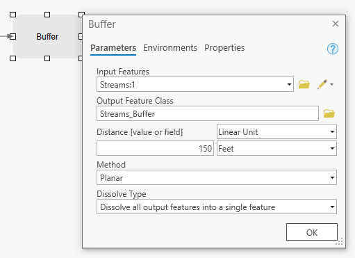
The Buffer tool window should now look similar to the preceding screenshot. Depending on what you may have done previously, the name of the input feature may be slightly different.
- Click OK once you have verified your settings.
- Click on the Auto Layout button on the ModelBuilder tab.
Your model should now include a single completed process that is in the ready to run state. You can tell it is ready to run because the tool and all lined variables are now displayed with a colored fill that is not gray, as shown in the following screenshot:

Now let's save your model to ensure your hard work is not lost in case something happens.
- Click on the Properties button in the Model group on the ModelBuilder tab.
- Fill in the following details in the respective properties:
- Type ParcelsStreamProtectionBuffer in Name field.
- Type Parcels Stream Protection Buffer Analysis in the Label field.
- Leave all other properties with default settings.
- Verify that your Tool Properties window looks like the following screenshot and then click OK:

- Click the Save button located in the Model group on the ModelBuilder tab to save the model. If you still have the Catalog pane open, you should see the name of the model change from model to the label that you entered previously.
The name for a model cannot contain spaces or other special characters with the exception of underscores. The label can be much more descriptive and does not have the same restrictions.
The process that you just created in the model will generate the buffer areas around the streams. Now you need to add another process that will calculate how much of each parcel is inside and outside that buffer area.
You will use the Union tool to union the parcels with the newly created stream buffer. This will create a new feature class that will split each parcel where it is overlapped by the stream buffer, thus allowing you to determine how much is inside and outside the buffer.
Step 3 – Adding another process
In this step, you will add another process to your model. This process will include the Union tool. You will then link this new process to the one that you created in the previous step:
- Click on the Tools button in the ModelBuilder tab again to open the Geoprocessing pane.
- Expand the Overlay toolset in the Analysis toolbox.
- Add the Union tool to your model by right-clicking on the tool and selecting Add to model.
- If required, using your scroll wheel, zoom out in the ModelBuilder window until you have room to see both the Union tool and the Buffer tool.
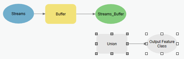
- With the Union tool and the Output Feature Class variable selected, use your mouse to move them so that they are located below the Buffer tool, as shown in the following screenshot:
You have now added the Union tool to the model. Now you need to link it to the output from the Buffer tool and define the rest of its required variables.
- Double-click on the Union tool to open the tool window.
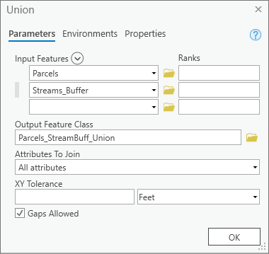
- In the Union tool window, click on the small arrow next to Input Features, and then select Parcels from the list that displays.
- Repeat this same process to select Streams_Buffer located under Model Variables.
- Set the output to C:StudentIntroArcProChapter12Ex12.gdbParcels_StreamBuff_Union.
- Verify that your Union tool settings match the following screenshot and click OK:
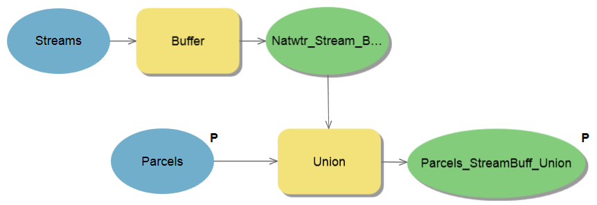
Your entire model should now be in the ready to run state and look similar to this:
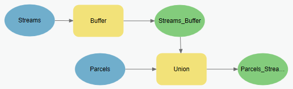
As compared to the preceding diagram, your layout may be different. That is acceptable as long as the proper connections are made, and the processes are in the ready to run state.
- Save your model and your project.
- You may close ArcGIS Pro or leave it open if you plan to continue.
You have learned how to create a model and have understood its components. After creating a model, of course, you will want to run it. There are many ways to run a model. So, we will look at how to run a model in the next section.
Running a model
You can run the entire model and the processes in the ready to run state or just a single process in the model. In this section, you will explore the different ways you can run a model you create in ModelBuilder.
If you wish to run the entire model, the easiest way to do that is simply double-click on it, from the toolbox it is stored in. This will run all processes in the model that are in the ready to run or have been run state. If you have allowed the users to provide values for some of the variables within the model, they will be prompted to enter those before the model is run.
Otherwise, if you did not allow for user input, the model will just indicate that there are no parameters in the geoprocessing window and all you need to do is click the Run button. You will learn how to make a model interactive a little later in this chapter.
You can also choose to run the model or processes in the model from the ModelBuilder window. Clicking on the Run button in the ModelBuilder tab will run all ready to run processes within the model. It will not run processes that are in the have been run or not ready to run state. This allows you to build and test a model as you go without being required to run the entire model.
Now that you know a little more about how to run a model, you will get to put that knowledge into practice.
Exercise 12B – Running a model
In this exercise, you will first run your model from within ModelBuilder. Then, you will get to run it directly from the toolbox so that you can see what your users will experience when they run the model.
Step 1 – Running the model from ModelBuilder
In this step, you will run the model that you created in Exercise 12A in Chapter 12, Automating Processes with ModelBuilder and Python, from within ModelBuilder. You will also explore how to run individual processes so that you can test your model as you create it:
- If you closed ArcGIS Pro after the last exercise, start ArcGIS Pro and open the Ex12.aprx project.
- Expand the Toolboxes folder in the Catalog pane and then expand the Ex12 toolbox.
- Right-click on the model that you created in Exercise 12A and select Edit from the displayed context menu. This will open the ModelBuilder window.
If you created your model successfully in the last exercise and saved it, all processes should be in the ready to run state. This is indicated by all tools and variables having a solid color fill applied. If any are filled with gray or empty, then you need to go back to Exercise 12Ain Chapter 12, Automating Processes with ModelBuilder and Python, and work back through the exercise.
- Right-click on the Buffer tool in ModelBuilder. Select Run to run the Buffer tool with the connected variables that you defined in the model. A small window will pop up inside ModelBuilder that displays the progress of the Buffer tool and will let you know when it completes. When the tool is finished, notice what happens to the graphics for the Buffer tool and its associated variables, as shown in the following screenshot:

The Buffer tool process is now in the has been run state. This means you have successfully run that process in the model.
As you are beginning to learn, the state of a process will impact how it runs. Now that this process is in the has been run state, it will not run again if you click the Run button in the ribbon. The Run button will only run those processes that are in the ready to run state. Let's verify that, though.
- Close the pop-up window that appeared when you ran the Buffer tool by clicking on the x located in the upper right corner.
- Click the Run button in the Run group on the ModelBuilder tab. Watch what happens to the model as it is run.
We will now move on to the next step about how to reset the run state.
Step 2 – Resetting the run state
In this step, you will learn how to reset the run state of all the processes in the model that are in the have been run state back to the ready to run state:
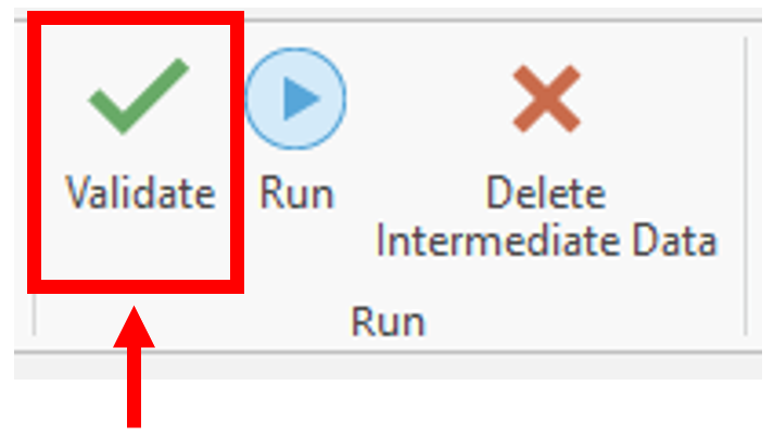
- Click on the Validate button in the Run group on the ModelBuilder tab in the ribbon as illustrated in the following screenshot:
- Click the Run button on the ribbon and watch how your model runs this time. All the processes will run this time because all of them are in the ready to run state.
Now you will actually verify that your model ran and created the feature classes that it was supposed to in the project database.
- Expand the Databases folder in the Catalog pane and then expand the Ex12 geodatabase.
If you do not see anything in the geodatabase, then you may need to right-click on it and select Refresh. That should allow it to display the new feature classes that your model has created.
- Right-click on each feature class that you see in the Ex12 geodatabase and select Delete until the database is empty. If you are asked whether you are sure that you want to permanently delete these items, select Yes. Deleting these feature classes will allow you to verify the model runs properly when you run it directly from the toolbox in the next step.
- Close the ModelBuilder window. If asked to save the model, do so.
We will now move onto the next step about how to run the model from a toolbox.
Step 3 – Running the model from a toolbox
In this step, you will now run the model directly from the toolbox. This will be how most users will access and run models that you create. Running the model using this method will allow you to have the same experience that your users will have when they run the model:
- Make sure the Map view is active by clicking on the Map tab at the top of the view area.
- In the Catalog pane, expand the Toolboxes | Ex12 toolbox.
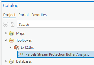
- Double-click on the Parcels Streams Protection Buffer Analysis model you created, as shown in the following screenshot:
- When you double-click on your model, it should open in the Geoprocessing pane. It will state that there are no parameters. This is expected because you have not defined any variables as parameters that will accept user input. Click the Run button at the bottom of the Geoprocessing pane.
- When the model is finished, return to the Catalog pane.
- Go to Databases | Ex12 geodatabase again.
When you ran the model from inside ModelBuilder, it produced two different feature classes within the Ex12 geodatabase. However, when you ran it from the toolbox, it only produced one. Why is that?
The answer is the feature class that was created by the Buffer tool in the model is considered intermediate data. Intermediate data is any feature class or table that is created within a model that is then used by other tools and is not a final result of a series of linked processes.
When you run a model from a toolbox, it will automatically clean up after itself. This means it automatically deletes the intermediate data that is created as the model runs. The only data it leaves is the final results of any processes in the model, which is not intermediate data. The end result is that you have the data that you need without also being left with a lot of partial datasets or layers that can clutter your database.
- Save your project and close ArcGIS Pro.
You have now learned how to run your model using various methods depending on where you are within the application. While creating or editing your model, you now know how to run individual processes that are included in the model. You also learned how to run your model from ModelBuilder and from a toolbox.
Now that you have created and run your first model, you can now run this model anytime you need to update the calculations for the areas of each parcel in and outside a floodplain.
We will learn how to make our model more interactive for the user in the next section.
Making a model interactive
So, you have created your first model. It is a very efficient tool that will help you quickly update information. However, what happens if the buffer distance changes or the director wants to look at different layers such as land use or just the commercial properties? In this section, you will explore different ways you can allow users to provide input for specified parameters included within your model.
Right now, the model you created is hardcoded to a specific set of variables. If something changes, you will be forced to edit the model before it can be used. Wouldn't it be more effective to allow others to specify different values for the variables in the model when they run it? You can allow that. It simply requires you to designate a variable as a parameter within the model. This allows the user to provide a value before they run the model.
To designate a variable as a parameter so that a user can specify a value when it is run, you simply right-click on the variable in ModelBuilder and select Parameter. When you do that, a small capital P will appear next to the variable indicating that it is now a model parameter, as illustrated in the following diagram:
In the preceding diagram, you can see that the Parcels and Parcels_ StreamBuff_Union variables are both marked as parameters. This will allow the user to select the values that they wish to use for those variables. This means they will be able to union the stream buffers with another layer besides just the parcels layer and control where the results are saved to and the name they are given.
Making a model interactive can greatly increase its functionality. It will allow the model to be used in different scenarios and with different datasets. The downside is that the more interactive you make a model, the greater the chance of introducing operator error. Users may select the wrong input layer for a tool or forget where they set the final results to be saved. This can result in more problems than the model was designed to solve. So, it is always a balancing act between flexibility and hard coding to eliminate error sources.
Now let's give you an opportunity to make your model interactive.
Exercise 12C – Allowing users to provide inputs to run models
The director was impressed with the model that you created. It allowed them to easily calculate the area of each parcel that was in and out of the stream protection area. The council is considering changing the buffer distance for the non-disturb area and the director wants to look at the impact of several different distances. So, they will need to be able to run the model in a way that allows them to specify different buffer distances and save the overall results with different names so that they can review the results of the different distances.
In this exercise, you will make the previous model you created interactive to those users and provide their own values to variables within the model. You will allow users to specify the buffer distance that they want to use and the final output of the model.
Step 1 – Marking variables as parameters
In this step, you will learn how to designate variables as parameters within a model. You will make the buffer distance and the output of the Union tool parameters within your model:
- Open ArcGIS Pro and the Ex12.aprx project.
- Expand the Toolboxes folder in the Catalog pane.
- Expand the Ex12 toolbox and right-click on the Parcels stream. Right-click on the Protection Buffer Analysis model you created in the previous exercise. Select Edit to open it in ModelBuilder.
- Right-click on the Output Variable for the Union tool and select Parameter. A small P should appear beside the variable, as shown in the following screenshot:

- Then, save your model.
By making the output of the Union tool a model parameter, users will now be able to choose where they will save the final output of the model and what it will be named. This is one of the two requirements that the director asked for. Now you need to allow users to specify a buffer distance.
The buffer distance is currently hardcoded into the model. You need to make it a parameter as you did the output of the Union tool. However, the buffer variable is hidden. So, first, you will need to make it visible within the model and then designate it as a parameter.
Step 2 – Exposing hidden variables
In this step, you will expose the distance variable for the Buffer tool so that you can make it a parameter:
- Right-click on the Buffer tool in ModelBuilder.
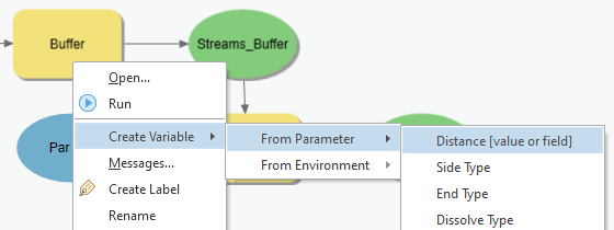
- Select the Create Variable | From Parameter option. This will display a list of all the hidden variables associated with the Buffer tool.
- Select Distance [value or field], as shown in the next screenshot:
The Distance variable should now be visible in your model. Now that it is visible you will be able to designate it as a parameter.
- Move your mouse pointer so that it is over the Distance variable that you just added to our model. When your pointer changes to two crossed arrows, indicating that it is now in move mode, drag the Distance variable so it is above the Buffer tool, as shown in the following screenshot:

- Right-click on the Distance variable and select Parameter. The small capital P should now appear next to the Distance variable, indicating it is now a model parameter.
- Save your model.
Your model should now look very similar to this:

The model shown in the preceding screenshot should now meet the requirements that the director asked for. They will now be able to use different distances from the streams and see the impact that it will have on the parcels. The director can save the result to a different name and location each time they run the model.
The last step is to verify your work. You need to test run the model to see whether it allows users to specify a distance and the output values.
Step 3 – Running the model
In this step, you will run the model from the toolbox to make sure it will allow the director to input a distance and specify where the output will be saved. Since you have not changed the overall logic or functionality of the model, there is no need to test the processes inside the model again:
- Close the ModelBuilder view.
- If needed, expand the Toolboxes folder and the Ex12 toolbox in the Catalog pane.
- Double-click on the model that you created to open it in the Geoprocessing pane.
Notice that this time when you open the model in the Geoprocessing pane, it looks different. Instead of saying no parameters, it is asking for user input. The user can provide values for the two variables that you designated as parameters.
- Change the value for the Parcels_Stream_Union variable to C:StudentIntroArcProChapter12Ex12.gdb%Your Name%_Results (that is, Tripp_Results).
- Change the Distance value to any value that you wish that is not 150 feet. You can even change the units if you desire.
- After you are done changing the values of the variables, click the Run button at the bottom of the Geoprocessing pane.
- Once the model has finished running, close the Geoprocessing pane.
- In the Catalog pane, verify that the resulting output feature class is in Ex12.gdb.
- Save your project and close ArcGIS Pro.
You have now created your first interactive model. This model provides more flexibility for the user, allowing them to investigate different scenarios. Next, you will be introduced to Python, which is the primary scripting language for the ArcGIS platform. You can use Python scripts to automate processes and then schedule them to run at specific times. Python scripts can also be used to help integrate ArcGIS with other applications. This makes the Python scripting language a powerful tool for increasing the effectiveness of your GIS.
Learning about Python
Python is the primary scripting language for the ArcGIS platform. It has replaced others, such as Visual Basic (VB). ArcGIS Pro 2.5 is currently compatible with Python 3.6.9, which is automatically installed when you install ArcGIS Pro.
Python has been fully integrated with the ArcGIS Geoprocessing Application Programming Interface (API) via the ArcPy module. This means you can use the geoprocessing tools from within ArcGIS Pro within your scripts, allowing you to automate and schedule tasks.
Unlike ModelBuilder, Python is not limited to just the ArcGIS platform. It is used to create scripts that access functions in other applications, the operating system, and the computer. This gives you the ability to create scripts that extend and integrate ArcGIS Pro's functionality across platforms and applications. As a result, Python is a very versatile tool in the GIS developer's arsenal.
Python scripts can be stored within ArcGIS Toolboxes or in standalone folders as .py files. Unlike other programming languages such as C++ or VB, creating Python scripts doesn't require special application development software. You can use simple text editors such as Notepad or WordPad. There are several free Integrated Development Environment (IDE) applications for Python, such as PythonWin or IDLE. IDE applications provide a better development environment over text editors because they include automatic coding hints and debugging tools. When you install ArcGIS, it automatically installs Python and IDLE.
ArcGIS Pro also includes a Python window that can be used to write Python scripts, run tools using Python, and load Python scripts to view code. New Python developers often find the Python window helpful because of its integrated interface and its autosuggest function, which helps guide proper syntax.
Let's look at some Python basics first.
Understanding Python basics
Since this is your first introduction to Python, it is a good time to introduce some fundamentals and best practices. These will serve you well as you begin to write your own scripts.
Commenting and documenting your scripts
When you begin creating a Python script, it is considered a best practice to include documentation within the code that will help other developers understand what is happening within the code and the purpose-specific parts of the script. This can also prove helpful for yourself if you have to come back to a script that you wrote some time ago and need to make changes.
This in-code documentation is traditionally accomplished using commenting. Think of commenting code as a form of metadata stored within the code itself. It provides users and other programmers with the who, what, where, when, and why data. They may need this data to successfully use, integrate, or edit a script that you create. Different programming languages use different methods to comment code. Python uses the pound sign (#) to identify comment lines within its code, as illustrated in the following screenshot:
As you can see in the preceding screenshot, anytime Python encounters a line that starts with a #, it ignores that line and moves to the next. It will keep ignoring lines until it encounters one that does not have a # at the beginning.
Traditionally, the first group of lines in a Python script is used to provide basic information about the script, such as its purpose, who created it, when was it created, what ArcGIS version it was created for, and so on. Providing this basic information is considered an industry best practice.
Now let's learn about the variables that we use in Python.
Learning about variables
Like a model, a Python script can contain variables. When you define a variable in Python, you give it a name and a value. Also similar to a model, the value assigned to a variable can be hardcoded, can reference the result of another process, or can be a function of ArcPy or another module.
For example, you could define a variable that would be used as an input for the Buffer tool as follows:
In_buf_fc = "streams"
This variable would then be used by the Buffer tool in a Python script as follows:
Buffer_analysis (In_buf_fc, "C:\GIS\Trippville.gdb\Streams_Buffer",
    "125 Feet", "FULL", "ROUND")
You can see from the preceding sample code, the use of the defined variable has been highlighted. In an actual script, you would not embolden the variable. That was just done in this example to help you see the use of the variable more easily.
Another particularly important thing to keep in mind when writing scripts is that Python is case sensitive. This means a variable named Mapsize is not the same as one named mapsize. To Python, those are two different and distinct objects. This is one of the most common causes of problems when writing and running Python scripts.
Python also has other restrictions when defining a variable within a script:
- Variable names must start with a letter. They cannot start with a number.
- Variable names cannot include spaces or other special characters. The one exception is an underscore ( _ ).
- Variable names cannot include reserved keywords such as the following:
- Class
- If
- For
- While
- Return
Now let's move on to learning about data paths used in Python.
Understanding data paths
Often when you define a variable, access data, or save the results of a tool, you need to reference a specific file or data path. In a traditional Windows environment, this typically requires you to define the path using backslashes. For example, you have been accessing the data and exercises for this book by going to C:StudentIntroArcPro. This is an example of a path.
Unfortunately, you cannot use this common method of defining a path within a Python script. Backslashes are reserved characters within Python that are used to indicate an escape or line continuation. So, when specifying a data path, you must use a different method. Python supports three methods for defining a path:
- Double backslashes: C:\Student\IntroArcPro
- Single forward slash: C:/Student/IntroArcPro
- Single backslash with an r in front of it: r"C:StudentIntroArcPro"
You can use either of the preceding methods when creating your own scripts. While it is acceptable to use any of these within a single script, it is recommended that you try to use the same method throughout the entire script. This will help you locate possible errors and fix them more quickly.
Let's learn about the ArcPy module in the next section.
Learning about the ArcPy module
The ArcPy module is a Python site package that allows Python access to ArcGIS functionality. The level of functionality is limited to the ArcGIS Pro license level and extensions available to the user running the script.
Through the ArcPy module, Python can not only be used to perform geoprocessing tasks using tools in ArcGIS Pro system toolboxes or other custom tools, but it can also execute other functions, such as listing available datasets within a given location or describing an existing dataset. It can also create objects, such as points, lines, polygons, extents, and more.
The ArcPy module contains several sub-modules. These sub-modules are specific purpose libraries containing functions and classes. These sub-modules include the following:
- Data access module (arcpy.da)
- Mapping module (arcpy.mp)
- Spatial Analyst module (arcpy.sa)
- Network Analyst module (arcpy.na)
The ArcPy module must be loaded into a script in order for Python to access ArcGIS Pro functionality. This is typically done at the very beginning of a new script using the following syntax:
import arcpy
This one line allows Python to access ArcGIS Pro tools and functions. Additional modules can also be loaded using that same line, such as the operating system (os) or system (sys) modules.
Now that you have a very basic understanding of the ArcPy module, how do you know the proper syntax for using geoprocessing tools in a Python script? In the next section, you will find out how to locate the proper syntax for the various geoprocessing tools included in ArcGIS Pro.
Locating Python syntax for a geoprocessing tool
Finding the Python code needed to execute a specific geoprocessing tool is as easy as opening the help information for the tool. Esri has included sample Python code for all the geoprocessing tools in ArcGIS Pro and its extensions.
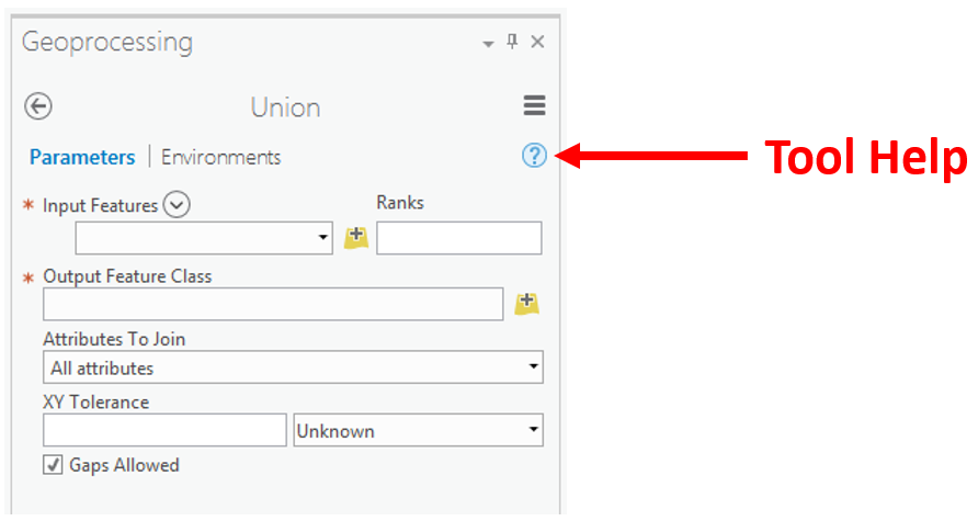
This includes the proper syntax to use within a script along with a description of the variables that can be used with the tool. Help for a specific tool can be accessed in the Geoprocessing pane when the tool is opened by clicking on the small blue question mark located on the upper right side of the pane, as shown in the following screenshot:
The Syntax page in the help information will show you the proper format for the code along with a description of the possible variables that may be included. The following screenshot shows an example of the syntax for the Union tool from the Esri help:

Help for all tools in ArcGIS Pro can be accessed from the ArcGIS Pro help online via the Tool Reference. The address to access it is http://pro.arcgis.com/en/pro-app/tool-reference/main/arcgis-pro-tool-reference.htm.
The help will also include code sample snippets that help put the syntax into context with a larger process. It is often possible to copy the sample code from the help and then paste it into your script; then, you can easily adjust the copied code to meet your needs, as shown in the following screenshot:

The preceding screenshot is an example of a sample code snippet for the Union tool that is found in the help. As you can see, it provides an understandable example of the code in a real-world context. This provides a much better understanding of how the tool can be used within a custom script you might create. Notice the comments included within the code sample and how they help to provide a better understanding of the purpose of the various parts of the code.
Now it is time for you to try your hand at writing a simple Python script.
Exercise 12D – Creating a Python script
The city of Trippville operates a GIS web application that allows citizens and elected officials to access parcel data. This GIS web application combines data from the city with other data layers from ArcGIS Online and Google Maps. As a result, the parcels must be projected from the local state plane coordinate system to the WGS 84 Web Mercator (Auxiliary Sphere) system. This is the common coordinate system used by Esri, Google, and Bing for GIS web applications and data.
You can also update the Acres field as new parcels that are added or combined before the new data is added to the web application. You can use the Calculate Field tool to accomplish this with an expression that converts the Shape_Length field, which is in feet, to acres.
In the past, you have manually performed these operations. However, you will be going on vacation and the director wants the parcel data to still be updated regularly while you are gone. They can copy the data to the web application but do not know how to perform the other operations. So, they want you to create an automated routine that can perform these operations automatically on a regular schedule.
Since the director wants this routine to run on an automated schedule, you will need to write a Python script. A model will not work in this case. In this exercise, you will write a basic Python script that will calculate the acreage of each parcel, update the Acres field, and then project the data from the state plane coordinate system that is currently in the WGS 84 Web Mercator (Auxiliary Sphere).
Step 1 – Opening IDLE
In this step, you will open the IDLE application so that you can begin creating your script:
- Click on your Start button. This is normally located in the lower-left corner of your screen in your taskbar. In Windows 8.1 or Windows 10, it appears as just four white squares.
- In Windows 8.1 or 10, click the small downward-pointing arrow to access all installed programs or apps.
- Navigate to the ArcGIS program group in the list of all programs. In Windows XP or Windows 7, you may need to expand the group to see the programs inside.
- Locate the IDLE (Python GUI) application and click on it to launch the program.
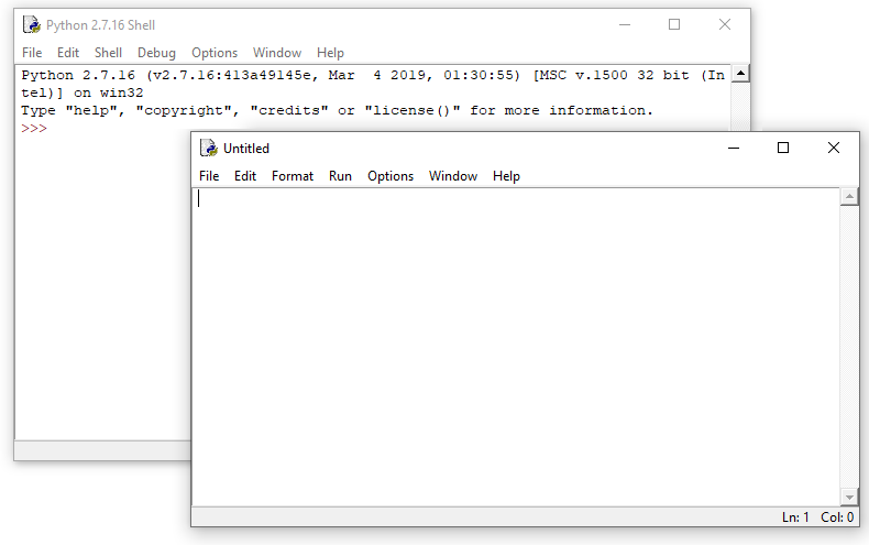
You have now opened the Python IDLE application. You will write your script within this application. It will open with the shell window.
The shell window displays messages and errors generated by a script when it is run from IDLE. You do not actually write scripts within this window. You will need to open a new code window to begin writing the script.
- Click the File | New File option. This will open the code window that you will use to write your script. You should now be able to see something like this:
- Click Options in the top menu and select Configure IDLE. You can do this in either of the IDLE windows.
- Click on the General tab and set Default Source Encoding to UTF-8 as shown in the following screenshot:
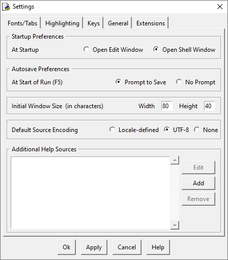
- Click Apply and Ok.
Now that you have configured your IDLE options, it is time to start writing a script.
Step 2 – Writing the script
Now you will begin writing the script that you need to accomplish the tasks you performed manually before. To start, you will insert some basic information concerning your script in accordance with best practices. Then, you will import the ArcPy module, and lastly, you will write the code for the script:
- First, you will save your empty script, so that it has a name. In the Untitled window, click on the File | Save option.
- In the Save As window, navigate to C:StudentIntroArcProChapter12, name your file AcresWebProject.py, and click Save.
You have just saved your empty script. You should see the new name and path shown at the top of the code window.
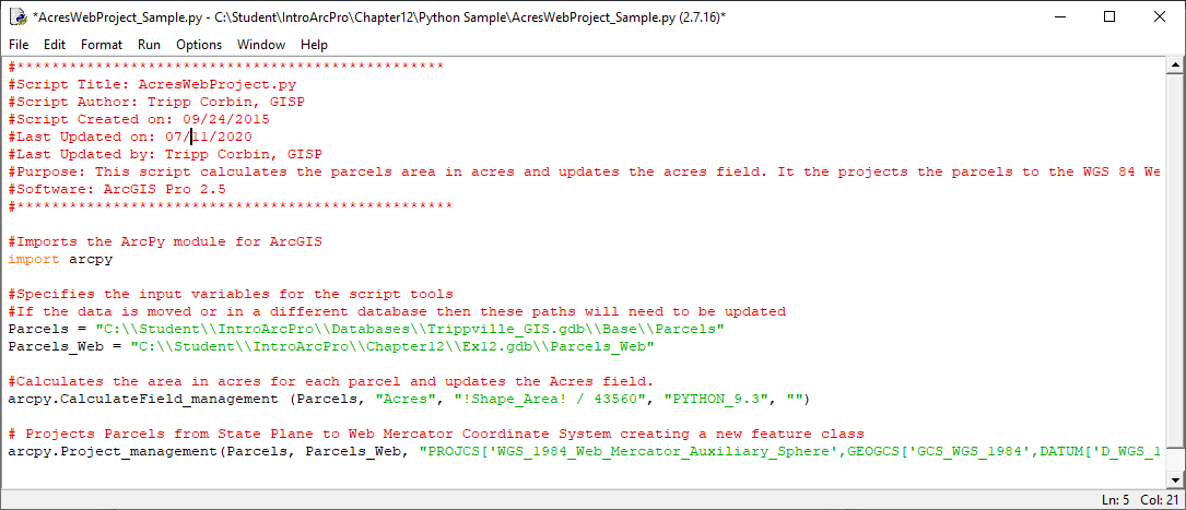
- Now you will add the general information at the beginning of the script as comments. Remember that # identifies a comment within Python code. Type the following example code into the IDLE code window (the Purpose part should all be typed on a single line; if you split it on to multiple lines, you will need to place # at the start of each line):
#**********************************************
#Script Title: AcresWebProject.py
#Script Author: Your Name
#Script Created on: Today's date
#Last Updated on: Today's date
#Last Updated by: Your Name
#Purpose: This script calculates the parcels area in acres and updates the acres field. It then projects the parcels to the WGS 84 Web Mercator coordinate system so it can be used within the City's web application.
#Software: ArcGIS Pro 2.5 (or the version you are running)
#*****************************************************
- Now you need to add the code line that imports the ArcPy module so that the script can access the ArcGIS Pro tools. Add the following code to your script in the code window:
#Imports the ArcPy module for ArcGIS
import arcpy
- Save your script by clicking File and then Save. If you get a warning, just click OK.
Now you will define some variables within your script that specify the location of the parcels data and where to save the results of the Project tool.
- Type the following code after the import statement in the code window:
#Specifies the input variables for the script tools
#If the data is moved or in a different database then these paths will need to be updated
Parcels = "C:\Student\IntroArcPro\Databases
    \Trippville_GIS.gdb\Base\Parcels"
Parcels_Web = "C:\Student\IntroArcPro\Chapter12\Ex12.gdb
     \Parcels_Web"
The preceding code you have just added to your Python script starts with two lines of comments which explain what the next lines do. As you have learned, comment lines are indicated with the # symbol. The next two lines define two variables.
The first is Parcels. This variable points to the location of the Parcels feature class, that is stored in the Base feature dataset within the Trippville_GIS geodatabase. The second variable you have defined in this code is Parcels_Web. It references the Parcels_Web feature class in the Ex12 geodatabase.
- Save your script.
Now you need to begin adding the code for the tools that you will need to run in the script. You will use the ArcGIS Pro help to get the proper syntax for the Calculate Field and Project tools. Then, modify it so that it works properly in your script.
- Open ArcGIS Pro and Ex12.aprx.
- Click on the Analysis tab and the Tools button to open the Geoprocessing pane.
- In the Geoprocessing pane, click on Toolboxes located near the top of the pane.
- Expand the Data Management Tools toolbox and the Fields toolset.
- Select the Calculate Field tool.
- Click on the Help button. It is the blue question mark in the upper right corner.
- You have opened the online tool reference for this tool; click on Syntax.
- Highlight and copy the syntax for the tool. It should read as follows:
CalculateField_management (in_table, field, expression,
    {expression_type}, {code_block})
- Active the IDLE code window and paste the copied syntax onto a line below the variables that you defined earlier.
- Add a comment above the code that you just pasted into the script that says calculates the area in acres for each parcel and updates the acres field.
- Now edit the code sample syntax that you just pasted into the script as follows:
arcpy.CalculateField_management (Parcels, "Acres", "!Shape_Area! /
    43560", "PYTHON_9.3", "")
- You have now defined the CalculateField tool within a Python script, so it includes all the variables it needs to run; save your script.
- Now you need to add the Project tool to the script and define its syntax properly. Using the same process that you used for the Calculate Field tool, open the help for the Project tool and copy the syntax into your script. The Project tool is located in the same toolbox but is in the Projections and Transformations toolset.
- Add an appropriate comment to the script that is above the code for the project tool, which will let others know its purpose similar to the comment that you added for the Calculate Field tool.
- Modify the Project tool code as follows (to make things easier you can copy the syntax from the Project Tool Sample.txt file in the Chapter12 folder):
arcpy.Project_management(Parcels, Parcels_Web, "PROJCS['WGS_1984_Web_Mercator_Auxiliary_Sphere',
GEOGCS['GCS_WGS_1984',DATUM['D_WGS_1984',SPHEROID['WGS_1984',6378137.0,298.257223563]],PRIMEM['Greenwich',0.0],UNIT['Degree',0.0174532925199433]],PROJECTION['Mercator_Auxiliary_Sphere'],PARAMETER['False_Easting',0.0],PARAMETER['False_Northing',0.0],PARAMETER['Central_Meridian',0.0],PARAMETER['Standard_Parallel_1',0.0],PARAMETER['Auxiliary_Sphere_Type',0.0],UNIT['Meter',1.0]]", "WGS_1984_(ITRF00)_To_NAD_1983", "PROJCS['NAD_1983_StatePlane_Georgia_West_FIPS_1002_Feet',GEOGCS['GCS_North_American_1983',DATUM['D_North_American_1983',SPHEROID['GRS_1980',6378137.0,298.257222101]],PRIMEM['Greenwich',0.0],UNIT['Degree',0.0174532925199433]],PROJECTION['Transverse_Mercator'],PARAMETER['False_Easting',2296583.333333333],PARAMETER['False_Northing',0.0],PARAMETER['Central_Meridian',-84.16666666666667],PARAMETER['Scale_Factor',0.9999],PARAMETER['Latitude_Of_Origin',30.0],UNIT['Foot_US',0.3048006096012192]]")
The preceding code seems extremely complicated, and to some extent it is. It contains all the parameters required to define two coordinate systems. The first is the coordinate system for the Parcels feature class. The second is the coordinate system used by the output feature class, Parcels_Web.
- Save your script.
Your script should look like this on your screen:
- Once you have verified your script and saved it, close IDLE.
We'll now move on to the next step.
Step 3 – Adding the script to ArcGIS Pro and running it
Now that you have created a Python script, you need to add it to ArcGIS Pro and test it. In this step, you will add the script you just created to a toolbox in your project and then run it:
- If necessary, start ArcGIS Pro and open Ex12.aprx.
- In the Catalog pane, expand the Toolboxes folder.
- Right-click on the Ex12 toolbox and select New>Script from the menu.
- Fill out the information for the new script as follows:
- Type CalcAcresProject in theNamefield.
- Type Calculate Parcel Acres and Project to Web Mercator in the Label field.
- Click on the Browse button located next to the Script File cell, then navigate to C:StudentIntroArcProChapter12, and select the AcresWebProject.py script that you just created. Your window should now look like this:

- Click OK once you have verified everything is set correctly.
The script will appear in the Ex12 toolbox. This means you can now run it in ArcGIS Pro. You must add all Python scripts that you create to a toolbox before they are able to be used in ArcGIS Pro. For those with experience with ArcGIS for Desktop, it should be noted that ArcGIS Pro does not support Python add-ins yet. That functionality should be added to a future version.
Now you will need to run the script to test and make sure it works as expected.
- Double-click on the Python script that you just added to the toolbox. This will open it in the Geoprocessing pane. Since you hardcoded all the variables into the script, it has no parameters that the user needs to define.
- Click the Run button at the bottom of the Geoprocessing pane.
- Once the script has completed running, return to the Catalog pane.
- Expand the Databases folder and expand Ex12.gdb. If the script ran successfully, you should see a new feature class named Parcels_Web. You may need to right-click on the Ex12 geodatabase and refresh in order to see the new feature class that was created.
If you do see the new feature class, congratulations! You have just created and run your first Python script. If your script did not run successfully, you may wish to compare it to the sample included in the Python Sample folder located in C:StudentIntroArcProChapter12.
- Save your project and close ArcGIS Pro along with IDLE, if it is still open.
You have just created your first Python script, which projects data from one coordinate system to another. Since this is a Python script, you could use the scheduling functionality found in your operating system to schedule this script to run at a specified frequency automatically so you do not have to worry about it. This can reduce your overall workload and ensure that required functions run on a regular schedule.
Summary
In this chapter, you learned that ArcGIS Pro contains two methods for automating and streamlining tasks; that is, you can create a model or a Python script. Which one will work best will largely depend on your skills and how they will be used. You have gained the skills to create and run your own model.
We learned that models are created in ModelBuilder, which provides a graphical interface for creating tools that will automate a series of processes required to accomplish an analysis or other workflow. Each model will contain a series of processes. Each process will include a tool that can be a geoprocessing tool, script, or another model, along with their associated variables. As you create a model, you can choose to make it interactive by designating variables as parameters. The biggest limitation of models is that they can only be run from inside of ArcGIS Pro. This means they cannot be scheduled to run automatically.
Python scripts can be used to automate processes that can then be scheduled to run at specified times and dates. Unlike the case with models, creating Python scripts does require knowledge of the Python language and the ability to write code.
In addition to the ability of Python scripts to be run on a schedule, they can also be used to access functionality from other applications other than ArcGIS Pro. Through this chapter, you have gained the skills to create scripts that can integrate the functionality of several different applications into a single automated script.
In the next chapter, you will learn how you can share the various maps and data you create in ArcGIS Pro with others on your computer network and those that are not on your network. You will also learn ways to share your GIS content with others that do not have GIS software.
Further reading
If you would like to learn more about creating Python scripts for ArcGIS, you might want to get Programming ArcGIS with Python Cookbook by Eric Pimpler.