Mathematics
In this chapter:
– Probability
– Perlin noise
– The map() function
– Trigonometry
– Recursion
– Two-dimensional arrays
Here we are. The fundamentals are finished, and I am going to start looking at some more sophisticated topics in Processing. You may find there is less of a story to follow from chapter to chapter. Nonetheless, although the concepts do not necessarily build on each other as fluidly as they did previously, the chapters are ordered with a step-by-step learning approach in mind.
Everything I do from here on out will still employ the same flow structure of setup() and draw(). I will continue to use functions from the Processing library and algorithms made of conditional statements and loops, and organize sketches with an object-oriented approach in mind. At this point, however, the descriptions will assume a knowledge of these essential topics, and I encourage you to return to earlier chapters to review as needed.
13-1 Mathematics and programming
Did you ever start to feel the sweat beading on your forehead the moment your teacher called you up to the board to write out the solution to the latest algebra assignment? Does the mere mention of the word “calculus” cause a trembling sensation in your extremities?
Relax; there is no need to be afraid. There is nothing to fear but the fear of mathematics itself. Perhaps at the beginning of reading this book, you feared computer programming. I certainly hope that, by now, any terrified sensations associated with code have been replaced with feelings of serenity, if not outright joy. This chapter aims to take a relaxed and friendly approach to a few useful topics from mathematics that will help you along the journey of developing Processing sketches.
You know, you have been using math all along.
For example, you have likely had an algebraic expression on almost every single page since learning variables.
float x = width/2;
And most recently, in Chapter 10, you tested intersection using the Pythagorean Theorem.
float d = dist(x1, x2, y1, y2);
These are just a few examples you have seen so far, and as you get more and more advanced, you may even find yourself online, late at night, googling “Sinusoidal Spiral Inverse Curve.” For now, I will start with a selection of useful mathematical topics.
13-2 Modulus
Let’s begin with a discussion of the modulo operator, written as a percent sign, in Processing. Modulus is a very simple concept (one that you learned without referring to it by name when you first studied division) that is incredibly useful for keeping a number within a certain boundary (a shape on the screen, an index value within the range of an array, etc.) The modulo operator calculates the remainder when one number is divided by another. It works with both integers and floats.
20 divided by 6 equals 3 remainder 2. (In other words 6 times 3plus 2 equals 20.)
therefore:
20 modulo 6 equals 2 or 20 % 6 = 2
Here are a few more, with some blanks for you to fill in.
| 17 divided by 4 equals 4 remainder 1 | 17 % 4 = 1 |
| 3 divided by 5 equals 0 remainder 3 | 3 % 5 = 3 |
| 10 divided by 3.75 equals 2 remainder 2.5 | 10 % 3.75 = 2.5 |
| 100 divided by 50 equals _________ remainder _________ | 100 % 40 _________ |
| 9.25 divided by 0.5 equals _________ remainder _________ | 9.25 % 0.5 _________ |
You will notice that if A = B % C, A can never be larger than C. The remainder can never be greater than or equal to the divisor.
Therefore, modulo can be used whenever you need to cycle a counter variable back to zero. The following lines of code:
x = x + 1;
if (x >= limit) {
x = 0;
}
can be replaced by:
x = (x + 1) % limit;
This is very useful if you want to count through the elements of an array one at a time, always returning to zero when you get to the length of the array.

13-3 Random numbers
In Chapter 4, you were introduced to the random() function, which allowed you to randomly fill variables. Processing’s random number generator produces what is known as a “uniform” distribution of numbers. For example, I ask for a random number between 0 and 9, 0 will come up 10 percent of the time, 1 will come up 10 percent of the time, 2 will come up 10 percent of the time, and so on. I could write a simple sketch using an array to prove this fact. See Example 13-2.
Example 13-2
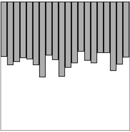
Figure 13-1
// An array to keep track of how often random numbers
are picked.
float[] randomCounts;
void setup() {
size(200, 200);
randomCounts = new float[20];
}
void draw() {
background(255);
// Pick a random number and increase the count
int index = int(random(randomCounts.length));
randomCounts[index]++ ;
// Draw a rectangle to graph results
stroke(0);
fill(175);
for (int x = 0; x < randomCounts.length; x++) {
rect(x * 10, 0, 9, randomCounts[x]);
}
}
With a few tricks, you can change the way you use random() to produce a nonuniform distribution of random numbers and generate probabilities for certain events to occur. For example, what if you wanted to create a sketch where the background color had a 10 percent chance of being green and a 90 percent chance of being blue?
13-4 Probability review
Let’s review the basic principles of probability, first looking at single event probability, that is, the likelihood of something to occur.
Given a system with a certain number of possible outcomes, the probability of any given event occurring is the number of outcomes which qualify as that event divided by total number of possible outcomes. The simplest example is a coin toss. There are a total of two possible outcomes (heads or tails). There is only one way to flip heads, therefore the probability of heads is one divided by two, that is, 1/2 or 50 percent.
Consider a deck of 52 cards. The probability of drawing an ace from that deck is:
number of aces/number of cards = 4/52 = 0.077 = ~8%
The probability of drawing a diamond is:
(number of diamonds) / (total cards) = 13/52 = 0.25 = 25%
You can also calculate the probability of multiple events occurring in sequence as the product of the individual probabilities of each event.
The probability of a coin flipping up heads three times in a row is:
(1/2) * (1/2) * (1/2) = 1/8 (or 0.125).
In other words, a coin will land heads three times in a row one out of eight times (with each “time” being three tosses).
Exercise 13-1
What is the probability of drawing two aces in a row from the deck of cards?
 ___________________________
13-5 Event probability in code
There are few different techniques for using the random() function with probability in code. For example, if I fill an array with a selection of numbers (some repeated), I can randomly pick from that array and generate events based on what I select.
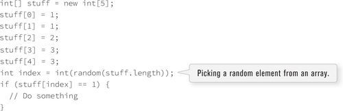
If you run this code, there will be a 40 percent chance of selecting the value 1, a 20 percent chance of selecting the value 2, and a 40 percent chance of selecting the value 3.
Another strategy is to ask for a random number (for simplicity, let’s consider random floating point values between 0 and 1) and only allow the event to happen if the random number picked is within a certain range. For example:
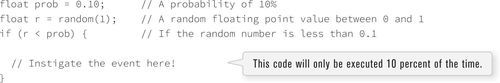
This same technique can also be applied to multiple outcomes.
Outcome A — 60 percent | Outcome B — 10 percent | Outcome C—30 percent
To implement this in code, I’ll pick one random float and check where it falls.
• Between 0.00 and 0.60 (60%) → outcome A
• Between 0.60 and 0.70 (10%) → outcome B
• Between 0.70 and 1.00 (30%) → outcome C
Example 13-3 draws a circle with a three different colors, each with the above probability (red: 60 percent, green: 10 percent, blue: 30 percent). This example is displayed in Figure 13-2.
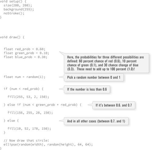
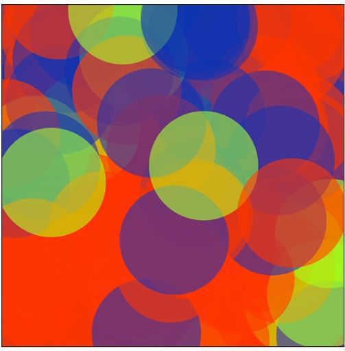
Figure 13-2
Exercise 13-2
Fill in the blanks in the following code so that the circle has a 10 percent chance of moving up, a 20% chance of moving down, and a 70 percent chance of doing nothing.
float y = 100;
void setup() {
size(200, 200);
}
void draw() {
background(0);
float r = random(1);
___________________________
___________________________
___________________________
___________________________
___________________________
___________________________
ellipse(width/2, y, 16, 16);
}
13-6 Perlin noise
One of the qualities of a good random number generator is that the numbers produced appear to have no relationship. If they exhibit no discernible pattern, they are considered random.
In programming behaviors that have an organic, almost lifelike quality, a little bit of randomness is a good thing. However, you might not want too much randomness. This is the approach taken by Ken Perlin, who developed a function in the early 1980s entitled “Perlin noise” that produces a naturally ordered (i.e., “smooth”) sequence of pseudo-random numbers. It was originally designed to create procedural textures, for which Ken Perlin won an Academy Award for Technical Achievement. Perlin noise can be used to generate a variety of interesting effects including clouds, landscapes, marble textures, and so on.
Figure 13-3 shows two graphs, a graph of Perlin noise over time (the x-axis represents time; note how the curve is smooth) compared to a graph of pure random numbers over time. (Visit this book’s website for the code that generated these graphs.)
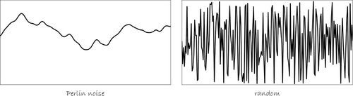
Figure 13-3
Processing has a built-in implementation of the Perlin noise algorithm with the function noise(). The noise() function takes one, two, or three arguments (referring to the “space” in which noise is computed: one, two, or three dimensions). This chapter will look at one-dimensional noise only. Visit the Processing website for further information about two-dimensional and three-dimensional noise.
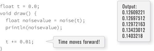
One-dimensional Perlin noise produces as a linear sequence of values over time. For example:
0.364, 0.363, 0.363, 0.364, 0.365
Note how the numbers move up or down randomly, but stay close to the value of their predecessor. Now, in order to get these numbers out of Processing, you have to do two things: (1) call the function noise(), and (2) pass in as an argument the current “time.” You would typically start at time t = 0 and therefore call the function like so: noise(t);
float t = 0.0;
float noisevalue = noise(t); // Noise at time 0
You can also take the above code and run it looping in draw().
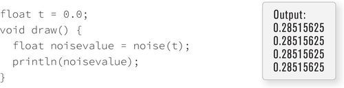
The above code results in the same value printed over and over. This is because I am asking for the result of the noise() function at the same point in time — 0.0 — over and over. If I increment the time variable t, however, I’ll get a different result.
How quickly you increment t also affects the smoothness of the noise. Try running the code several times, incrementing t by 0.01, 0.02, 0.05, 0.1, 0.0001, and so on.
By now, you may have noticed that noise() always returns a floating point value between 0 and 1. This detail cannot be overlooked, as it affects how you use Perlin noise in a Processing sketch. Example 13-4 assigns the result of the noise() function to the size of a circle. The noise value is scaled by multiplying by the width of the window. If the width is 200, and the range of noise() is between 0.0 and 1.0, the range of noise() multiplied by the width is 0.0 to 200.0. This is illustrated by the table below and by Example 13-4.


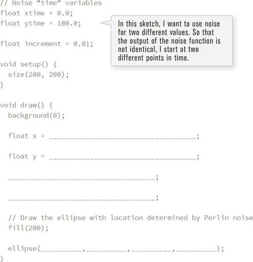
Exercise 13-3
Complete the following code that uses Perlin noise to set the location of a circle. Run the code. Does the circle appear to be moving “naturally”?
13-7 The map() function
Using Perlin noise values for setting a color or x-position was easy. If, say, the x-position for an ellipse ranges between 0 and width all I need to do is multiply the result of the noise function (which outputs a range between 0 and 1) by width.
float x = width * noise(t);
ellipse(x, 100, 20, 20);
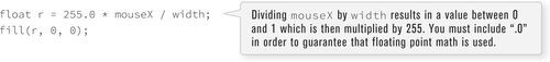
This range conversion is known as mapping. I mapped a Perlin noise value between 0 and 1 to an x-position between 0 and width. This sort of conversion comes up all the time in programming. Perhaps you want to map the mouse x-position (ranging between 0 and width) to a color value (ranging between 0 and 255). The math is a bit more complex but manageable.
Now let’s consider a more complex scenario. Let’s say you are reading values from a sensor that range between 65 and 324. And you want to map those values to a color range between 0 and 255. Now things are getting trickier. Fortunately, Processing includes a map() function that handles the math for converting values from one range to another. map() expects four arguments as listed below:
1. value: this is the value you want to map.
2. current min: the minimum of the value’s range.
3. current max: the maximum of the value’s range.
4. new min: the minimum of the new value’s range.
5. new max: the maximum of the new value’s range.
In the scenario I just described, the value is the sensor reading. The current min and max is the sensor’s range: 65 and 324. The new min and max is the range fill() expects: 0 and 255.
float r = map(sensor, 65, 324, 0, 255);
fill(r, 0, 0);
Using “min” and “max” to describe the new range isn’t exactly accurate. map() will happily invert the relationship as well. If you wanted the shape to appear red when the sensor value is low and black when it is high, you can simply swap the placement of 0 and 255.
float r = map(sensor, 65, 324, 255, 0);
fill(r, 0, 0);
Following is an example that demonstrates the map() function. Here the red and blue values of the background are tied to the mouse’s x and y positions.

Exercise 13-4: Rewrite your answer to Exercise 13-3 on page 244 using the map() function.
13-8 Angles
Some of the examples in this book will require a basic understanding of how angles are defined in Processing. In Chapter 14, for example, you will need to know about angles in order to feel comfortable using the rotate() function to rotate and spin objects.
In order to get ready for these upcoming examples, you need to learn about radians and degrees. It’s likely you’re familiar with the concept of an angle in degrees. A full rotation goes from zero to 360°. An angle of 90° (a right angle) is one-fourth of 360°, shown in Figure 13-5 as two perpendicular lines.
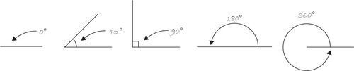
Figure 13-5
It’s fairly intuitive to think angles in terms of degrees. For example, the rectangle in Figure 13-6 is rotated 45° around its center.
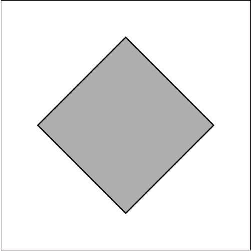
Figure 13-6
Processing, however, requires angles to be specified in radians. A radian is a unit of measurement for angles defined by the ratio of the length of the arc of a circle to the radius of that circle. One radian is the angle at which that ratio equals one (see Figure 13-7). An angle of 180° = π radians (π is the symbol for pi, more on this below.) An angle of 360° = 2π radians, and 90° = π/2 radians, and so on.
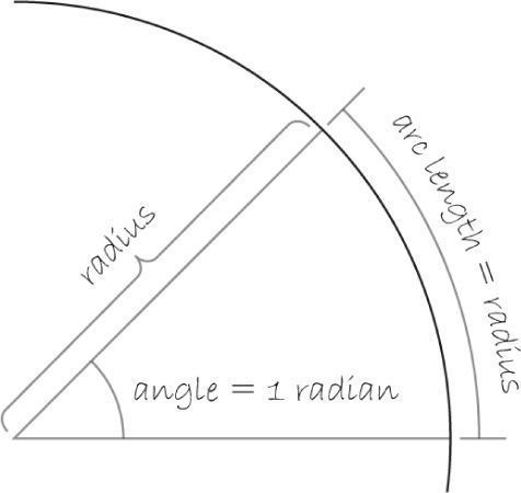
Figure 13-7
The formula to convert from degrees to radians is:
radians = 2π × (degrees ÷ 360)
Fortunately for us, if you prefer to think in degrees but code with radians, Processing makes this easy. The radians() function will automatically convert values from degrees to radians. In addition, the constants PI and TWO_PI are available for convenient access to these commonly used numbers (equivalent to 180° and 360°, respectively). The following code, for example, will rotate shapes by 60° (rotation will be fully explored in the next chapter).
float angle = radians(60);
Exercise 13-5
A dancer spins around two full rotations. How many degrees did the dancer rotate? How many radians?
Degrees: ____________ Radians: ____________
13-9 Trigonometry
Sohcahtoa. Strangely enough, this seemingly nonsense word, sohcahtoa, is the foundation for a lot of computer graphics work. Any time you need to calculate an angle, determine the distance between points, deal with circles, arcs, lines, and so on, you will find that a basic understanding of trigonometry is essential.
Trigonometry is the study of the relationships between the sides and angles of triangles and sohcahtoa is a mnemonic device for remembering the definitions of the trigonometric functions, sine, cosine, and tangent. See Figure 13-8.

Figure 13-8
• soh: sine = opposite/hypotenuse
• cah: cosine = adjacent/hypotenuse
• toa: tangent = opposite/adjacent
Any time you display a shape in Processing, you have to specify a pixel location, given as (x,y) coordinates. These coordinates are known as Cartesian coordinates, named for the French mathematician René Descartes, who developed the ideas behind Cartesian space.
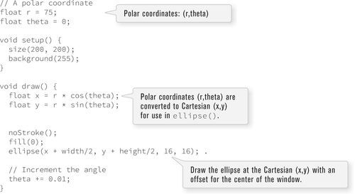
Another useful coordinate system, known as polar coordinates, describes a point in space as an angle of rotation around the origin and a radius from the origin. You can’t use polar coordinates as arguments to a function in Processing. However, the trigonometric formulas allow you convert those coordinates to Cartesian, which can then be used to draw a shape. See Figure 13-9

Figure 13-9
.
sine(theta) = y/r → y = sine(theta) × r
cosine(theta) = y/r → y = cosine(theta) × r
For example, assuming a radius r and an angle theta, I can calculate x and y using the above formula. The functions for sine and cosine in Processing are sin() and cos(), respectively. They each take one argument, a floating point angle measured in radians.
float r = 75;
float theta = PI / 4; // You could also say: float theta = radians(45);
float x = r * cos(theta);
float y = r * sin(theta);
This type of conversion can be useful in certain applications. For example, how would you move a shape along a circular path using Cartesian coordinates? It would be tough. Using polar coordinates, however, this task is easy. Simply increment the angle!
Here is how it’s done with global variables r and theta.

Exercise 13-6
Using Example 13-6, draw a spiral path. Start in the center and move outward. Note that this can be done by changing only one line of code and adding one line of code!

13-10 Oscillation
Trigonometric functions can be used for more than geometric calculations associated with right triangles. Let’s take a look at Figure 13-11, a graph of the sine function where y = sine(x).

Figure 13-11
You will notice that the output of sine is a smooth curve alternating between −1 and 1. This type of behavior is known as oscillation, a periodic movement between two points. A swinging pendulum, for example, oscillates.
I can simulate oscillation in a Processing sketch by assigning the output of the sine function to an object’s location. This is similar to how I used noise() to control the size of a circle (see Example 13-4), only with sin() controlling a location. Note that while noise() produces a number between 0 and 1.0, sin() outputs a range between −1 and 1. Example 13-7 shows the code for an oscillating pendulum.


Exercise 13-7
Encapsulate the above functionality into an Oscillator object. Create an array of Oscillators, each moving at different rates along the x and y axes. Here is some code for the Oscillator class to help you get started.
class Oscillator {
float xtheta;
float ytheta;
__________________________________________
Oscillator() {
xtheta = 0;
ytheta = 0;
________________________________________
}
void oscillate() {
________________________________________
________________________________________
}
void display() {
float x = ________________________________________
float y = ________________________________________
ellipse(x, y, 16, 16);
}
}
Exercise 13-8: Use the sine function to create a “breathing” shape, that is, one whose size oscillates.
I can also produce some interesting results by drawing a sequence of shapes along the path of the sine function. See Example 13-8.


Exercise 13-9: Rewrite the above example to use the noise() function instead of sin().
13-11 Recursion

In 1975, Benoit Mandelbrot coined the term fractal to describe self-similar shapes found in nature. Much of the stuff you encounter in the physical world can be described by idealized geometrical forms — a postcard has a rectangular shape, a ping-pong ball is spherical, and so on. However, many naturally occurring structures cannot be described by such simple means. Some examples are snowflakes, trees, coastlines, and mountains. Fractals provide a geometry for describing and simulating these types of self-similar shapes (by “self-similar,” I mean no matter how “zoomed out” or “zoomed in,” the shape ultimately appears the same). One process for generating these shapes is known as recursion.
You know that a function can call another function. You do this whenever you call any function inside of the draw() function. But can a function call itself? Can draw() call draw()? In fact, it can (although calling draw() from within draw() is a terrible example, since it would result in an infinite loop).
Functions that call themselves are recursive and are appropriate for solving different types of problems. This occurs in mathematical calculations; the most common example of this is “factorial.”
The factorial of any number n, usually written as n!, is defined as:
n! = (n − 1) × (n − 2) × (n − 3) … × 1
In other words, factorial is the product of all whole numbers from 1 to n. For example.
5! = 5 × 4 × 3 × 2 × 1
I could write a function to calculate factorial using a for loop in Processing:
int factorial(int n) {
int f = 1;
for (int i = 0; i < n; i++) {
f = f * (i + 1);
}
return f;
}
If you look closely at how factorial works, however, you will notice something interesting. Let’s examine 4! and 3!
4! = 4 × 3 × 2 × 1
3! = 3 × 2 × 1
therefore… 4! = 4 × 3!
Let’s describe this in more general terms. For any positive integer n:
n! = n × (n − 1)!
1! = 1
Written in English:
The factorial of n is defined as n times the factorial of (n − 1).
The definition of factorial includes factorial?! It’s kind of like saying “tired” is defined as “the feeling you get when you’re tired.” This concept of self-reference in functions is known as recursion. And you can use recursion to write a function for factorial that calls itself.
int factorial(int n) {
if (n == 1) {
return 1;
} else {
return n * factorial(n−1);
}
}
Crazy, I know. But it works. Figure 13-15 walks through the steps that happen when factorial(4) is called.
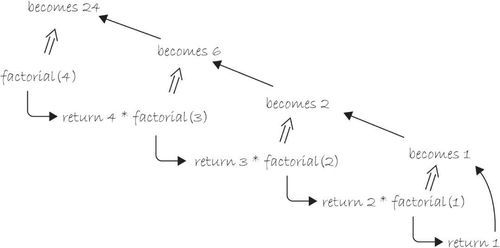
Figure 13-15
The same principle can be applied to graphics with interesting results. Take a look at the following recursive function. The results are shown in Figure 13-16.
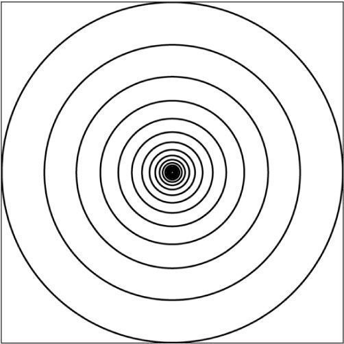
Figure 13-16
void drawCircle(int x, int y, float radius) {
ellipse(x, y, radius, radius);
if (radius > 2) {
radius * = 0.75;
drawCircle(x, y, radius);
}
}
What does drawCircle() do? It draws an ellipse based on a set of parameters received as arguments, and then calls itself with the same parameters (adjusting them slightly). The result is a series of circles each drawn inside the previous circle.
Notice that the above function only recursively calls itself if the radius is greater than two. This is a crucial point. All recursive functions must have an exit condition! This is identical to iteration. In Chapter 6, you learned that all for and while loops must include a boolean test that eventually evaluates to false, thus exiting the loop. Without one, the program would crash, caught inside an infinite loop. The same can be said about recursion. If a recursive function calls itself forever and ever, you will most likely be treated to a nice frozen screen.
The preceding circles example is rather trivial, since it could easily be achieved through simple iteration. However, in more complex scenarios where a method calls itself more than once, recursion becomes wonderfully elegant.
Let’s revise drawCircle() to be a bit more complex. For every circle displayed, draw a circle half its size to the left and right of that circle. See Example 13-9.
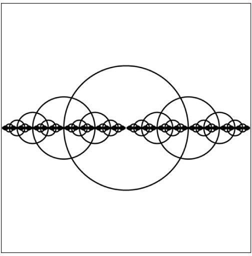
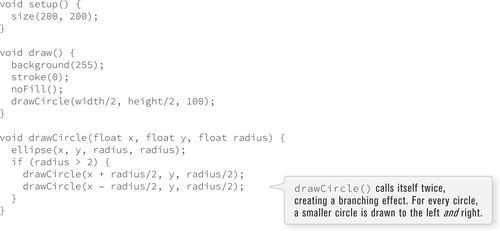
With a teeny bit more code, I can add a circle above and below. This result is shown in Figure 13-18.
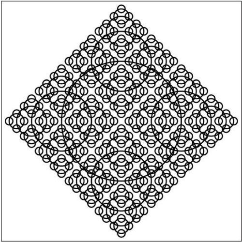
Figure 13-18
void drawCircle(float x, float y, float radius) {
ellipse(x, y, radius, radius);
if (radius > 8) {
drawCircle(x + radius/2, y, radius/2);
drawCircle(x − radius/2, y, radius/2);
drawCircle(x, y + radius/2, radius/2);
drawCircle(x, y − radius/2, radius/2);
}
}
Just try recreating this sketch with iteration instead of recursion! I dare you!
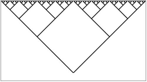
Exercise 13-10
Complete the code which generates the following pattern (Note: the solution uses lines, although it would also be possible to create the image using rotated rectangles, which you will learn how to do in Chapter 14).
void setup() {
size(400, 200);
}
void draw() {
background(255);
stroke(0);
branch(width/2, height, 100);
}
void branch(float x, float y, float h) {
__________________________________________________;
__________________________________________________;
if (____________________________) {
__________________________________________________;
__________________________________________________;
}
}
13-12 Two-dimensional arrays
In Chapter 9, you learned that an array keeps track of multiple pieces of information in linear order, a one-dimensional list. However, the data associated with certain systems (a digital image, a board game, etc.) lives in two dimensions. To visualize this data, you need a multi-dimensional data structure, that is, a multi-dimensional array.
A two-dimensional array is really nothing more than an array of arrays (a three-dimensional array is an array of arrays of arrays). Think of your dinner. You could have a one-dimensional list of everything you eat:
(lettuce, tomatoes, salad dressing, steak, mashed potatoes, string beans, cake, ice cream, coffee)
Or you could have a two-dimensional list of three courses, each containing three things you eat:
(lettuce, tomatoes, salad dressing) and (steak, mashed potatoes, string beans) and (cake, ice cream, coffee)
In the case of an array, an old-fashioned one-dimensional array looks like this:
int[] myArray = {0, 1, 2, 3};
And a two-dimensional array looks like this:
int[][] myArray = { {0, 1, 2, 3}, {3, 2, 1, 0}, {3, 5, 6, 1}, {3, 8, 3, 4} } ;
For me, it’s easier to think of the two-dimensional array as a matrix. A matrix can be thought of as a grid of numbers, arranged in rows and columns, kind of like a bingo board. I’ll write the two-dimensional array out as follows to illustrate this point:
int[][] myArray = { {0, 1, 2, 3},
{3, 2, 1, 0},
{3, 5, 6, 1},
{3, 8, 3, 4} };
To access an individual element of a two-dimensional array, you need two indices. The first specifies which array is the array of arrays and the second specifies which element of that array. Thus myArray[2] [1] is 5 (bolded above to illustrate this point).
Let’s use this type of data structure to encode information about an image. For example, the grayscale image in Figure 13-19 could be represented by the following array:

Figure 13-19
int[][] myArray = { {236, 189, 189, 0},
{236, 80, 189, 189},
{236, 0, 189, 80},
{236, 189, 189, 80} };
To walk through every element of a one-dimensional array, I’ll use a for loop, that is:
int[] myArray = new int[10];
for (int i = 0; i < myArray.length; i++) {
myArray[i] = 0;
}
For a two-dimensional array, in order to reference every element, I must use two nested loops. This provides a counter variable for every column and every row in the matrix. See Figure 13-20
int cols = 10;
int rows = 10;
int[][] myArray = new int[cols][rows];
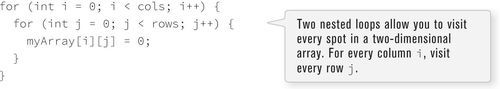
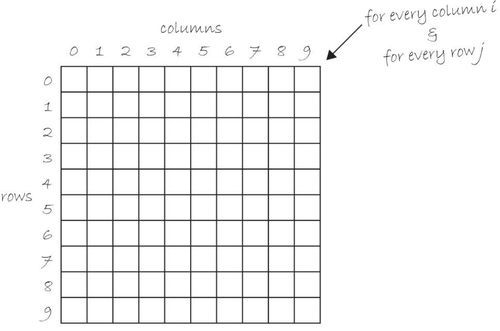
Figure 13-20
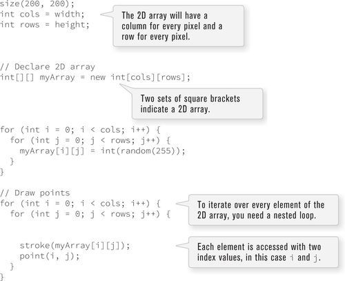
For example, you might write a program using a two-dimensional array to draw a grayscale image as in Example 13-10.

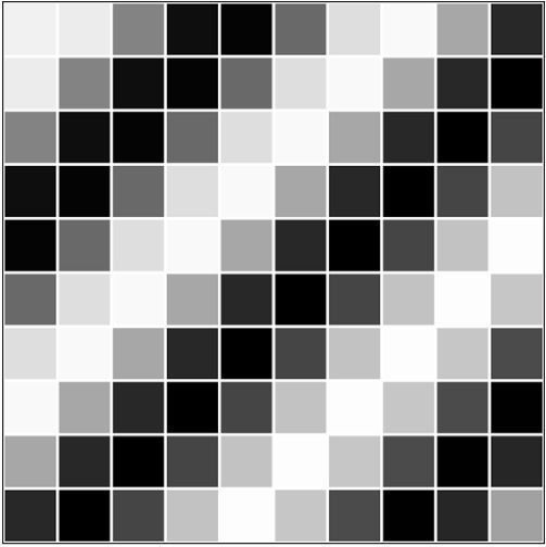
A two-dimensional array can also be used to store objects, which is especially convenient for programming sketches that involve some sort of “grid” or “board.” Example 13-11 displays a grid of Cell objects stored in a two-dimensional array. Each cell is a rectangle whose brightness oscillates from 0–255 with a sine function.

Exercise 13-11
Develop the beginnings of a Tic-Tac-Toe game. Create a Cell object that can exist in one of two states: O or nothing. When you click on the cell, its state changes from nothing to “O”. Here is a frame work to get you started.
Cell[][] board;
int cols = 3;
int rows = 3;
void setup() {
// What goes here?
}
void draw() {
background(0);
for (int i = 0; i < cols; i++) {
for (int j = 0; j < rows; j + +) {
board[i][j].display();
}
}
}
void mousePressed() {
// What goes here?
}
// A Cell object
class Cell {
float x, y;
float w, h;
int state;
// Cell Constructor
Cell(float tempX, float tempY, float tempW, float tempH) {
// What goes here?
}
void click(int mx, int my) {
// What goes here?
}
void display() {
// What goes here?
}
}
Exercise 13-12: If you are feeling saucy, go ahead and complete the Tic-Tac-Toe game adding X and alternating player turns with mouse clicks.