Images
Politics will eventually be replaced by imagery. The politician will be only too happy to abdicate in favor of his image, because the image will be much more powerful than he could ever be.
—Marshall McLuhan
When it comes to pixels, I think I’ve had my fill. There are enough pixels in my fingers and brains that I probably need a few decades to digest all of them.
—John Maeda
In this chapter:
– Displaying images
– Changing image color
– The pixels of an image
– Simple image processing
– Interactive image processing
A digital image is nothing more than data — numbers indicating variations of red, green, and blue at a particular location on a grid of pixels. Most of the time, we view these pixels as miniature rectangles sandwiched together on a computer screen. With a little creative thinking and some lower level manipulation of pixels with code, however, you can display that information in a myriad of ways. This chapter is dedicated to breaking out of simple shape drawing in Processing and using images (and their pixels) as the building blocks of Processing graphics.
15-1 Getting started with images
As you just learned in Section 14-10 on page 294, Processing has a bunch of handy classes all ready to go for your use. (Later, in Chapter 23, you will discover that you also have access to a vast library of Java classes.) While I only briefly examined PShape objects in Chapter 14, this chapter will be entirely dedicated to another Processing-defined class: PImage, a class for loading and displaying an image such as the one shown in Figure 15-1.

Figure 15-1
Just as with PShape, using an instance of a PImage object is no different than using a user-defined class. First, a variable of type PImage, named img, is declared. Second, a new instance of a PImage object is created via the loadImage() method. loadImage() takes one argument, a String (strings of text are explored in greater detail in Chapter 17) indicating a file name, and loads that file into memory. loadImage() looks for image files stored in your Processing sketch’s data folder.
The data folder: How do I get there?
Images can be added to the data folder automatically by dragging a file into your Processing window. You can also add files via:
Sketch → Add File…
or manually:
Sketch → Show Sketch Folder
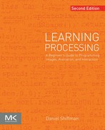
This will open up the sketch folder as shown in Figure 15-2. If there is no data directory, create one. Otherwise, place your image files inside. Processing accepts the following file formats for images: GIF, JPG, TGA, and PNG. You’ll want to make sure you include the file extension when referencing the file name as well, e.g., “file.jpg”.
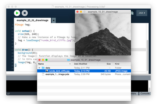
Figure 15-2
In Example 15-1, it may seem a bit peculiar that I never called a “constructor” to instantiate the PImage object, saying new PImage(). After all, in each of the object-related examples to date, a constructor is a must for producing an object instance.

Spaceship ss = new Spaceship();
Flower flr = new Flower(25);
And yet a PImage is created without new, using loadImage():
PImage img = loadImage(“file.jpg”);
In fact, the loadImage() function performs the work of a constructor, returning a brand new instance of a PImage object generated from the specified filename. You can think of it as the PImage constructor for loading images from a file. For creating a blank image, the createImage() function is used.
// Create a blank image, 200 × 200 pixels with RGB color
PImage img = createImage(200, 200, RGB);
I should also note that the process of loading the image from the hard drive into memory is a slow one, and you should make sure your sketches only have to do it once, in setup(). Loading images in draw() may result in slow performance, as well as “Out of Memory” errors. You should also avoid calling loadImage() above setup() as Processing will not yet know the location of the “data” folder and will report an error.
Once the image is loaded, it’s displayed with the image() function. The image() function must include three arguments — the image to be displayed, the x location, and the y location. Optionally, two arguments can be added to resize the image to a certain width and height.
image(img, 10, 20, 90, 60);
 Exercise 15-1: Load and display an image. Control the image’s width and height with the mouse.
15-2 Animation with an image
From here, it’s easy to see how you can use images to further develop examples from previous chapters. Note in the following example how I draw the image relative to its center using imageMode() which works similarly to rectMode() but is applied to images.
Figure 15-3

Exercise 15-2
Rewrite this example in an object-oriented fashion where the data for the image, location, size, rotation, and so on is contained in a class. Can you have the class swap images when it hits the edge of the screen?

15-3 My very first image processing filter
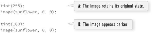
Every now and then, when displaying an image, you might like to alter its appearance. Perhaps you would like the image to appear darker, transparent, bluish, and so on. This type of simple image filtering is achieved with Processing’s tint() function. tint() is essentially the image equivalent of shape’s fill(), setting the color and alpha transparency for displaying an image on screen. An image, nevertheless, is not usually all one color. The arguments for tint() simply specify how much of a given color to use for every pixel of that image, as well as how transparent those pixels should appear.
For the following examples, assume that two images (a sunflower and a dog) have been loaded and the dog is displayed as the background (which will allow me to demonstrate transparency). See Figure 15.4. For color versions of these images visit http://www.learningprocessing.com.

Figure 15-4
PImage sunflower = loadImage("sunflower.jpg");
PImage dog = loadImage("dog.jpg");
background(dog);
If tint() receives one argument, only the brightness of the image is affected.
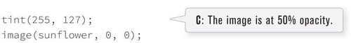
A second argument will change the image’s alpha transparency.
Three arguments affect the brightness of the red, green, and blue components of each color.

Finally, adding a fourth argument to the method manipulates the alpha (same as with two arguments). Incidentally, the range of values for tint() can be specified with colorMode() (see Chapter 1).

Exercise 15-3: Display an image using tint(). Use the mouse location to control the amount of red, green, and blue tint. Also try using the distance of the mouse from the corners or center.
Exercise 15-4: Using tint(), create a montage of blended images. What happens when you layer a large number of images, each with different alpha transparency, on top of each other? Can you make it interactive so that different images fade in and out?
15-4 An array of images
One image is nice, a good place to start. It will not be long, however, until the temptation of using many images takes over. Yes, you could keep track of multiple images with multiple variables, but here is a magnificent opportunity to rediscover the power of the array. Let’s assume I have five images and want to display a new background image each time the user clicks the mouse.
First, I’ll set up an array of images, as a global variable.
// Image array
PImage[] images = new PImage[5];
Second, I’ll load each image file into the appropriate location in the array. This happens in setup().
// Loading images into an array
images[0] = loadImage("cat.jpg");
images[1] = loadImage("mouse.jpg");
images[2] = loadImage("dog.jpg");
images[3] = loadImage("kangaroo.jpg");
images[4] = loadImage("porcupine.jpg");
Of course, this is somewhat awkward. Loading each image individually is not terribly elegant. With five images, sure, it’s manageable, but imagine writing the above code with 100 images. One solution is to store the filenames in a String array and use a for statement to initialize all the array elements.
// Loading images into an array from an array of filenames
String[] filenames = {"cat.jpg", "mouse.jpg", "dog.jpg", "kangaroo.jpg",
"porcupine.jpg");
for (int i = 0; i < filenames.length; i++) {
images[i] = loadImage(filenames[i]);
}
Even better, if I just took a little time out of my hectic schedule to plan ahead, numbering the image files (“animal0.jpg”, “animal1.jpg”, “animal2.jpg”, etc.), I could really simplify the code:
// Loading images with numbered files
for (int i = 0; i < images.length; i++) {
images[i] = loadImage("animal" + i + ".jpg");
}
Once the images are loaded, it’s on to draw(). There, I’ll choose to display one particular image, picking from the array by referencing an index (“0” below).
image(images[0], 0, 0);
Of course, hard-coding the index value is foolish. I’ll need a variable in order to dynamically display a different image at any given moment in time.
image(images[imageIndex], 0, 0);
The imagelndex variable should be declared as a global variable (of type integer). Its value can be changed throughout the course of the program. The full version is shown in Example 15-3.

To play the images in sequence as an animation, follow Example 15-4. (Only the new draw() function is included below.)

Exercise 15-5: Create multiple instances of an image sequence onscreen. Have them start at different times within the sequence so that they are out of sync. Hint: Use object-oriented programming to place the image sequence in a class.
15-5 Pixels, pixels, and more pixels
If you have been diligently reading this book in precisely the prescribed order, you will notice that so far, the only offered means for drawing to the screen is through a function call. “Draw a line between these points,” or “Fill an ellipse with red,” or “Load this JPG image and place it on the screen here.” But somewhere, somehow, someone had to write code that translates these function calls into setting the individual pixels on the screen to reflect the requested shape. A line does not appear because you say line(), it appears because all the pixels along a linear path between two points change color. Fortunately, you do not have to manage this lower-level-pixel-setting on a day-to-day basis. You have the developers of Processing (and Java) to thank for the many drawing functions that take care of this business.
Nevertheless, from time to time, you may want to break out of a mundane shape drawing existence and deal with the pixels on the screen directly. Processing provides this functionality via the pixels array.
You are familiar with the idea of each pixel on the screen having an (x,y) position in a two-dimensional window. However, the array pixels has only one dimension, storing color values in linear sequence. See Figure 15-5.
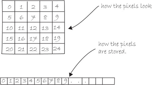
Figure 15-5
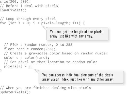
Take the following example. This sketch sets each pixel in a window to a random grayscale value. The pixels array is just like an other array, the only difference is that you do not have to declare it since it is a Processing built-in variable.

Figure 15-6
First, I should point out something important in the above example. Whenever you’re accessing the pixels of a Processing window, you must alert Processing to this activity. This is accomplished with two functions:
• loadPixels() — This function is called before you access the pixel array, saying “load the pixels, I would like to speak with them!”
• updatePixels() — This function is called after you finish with the pixel array, saying “Go ahead and update the pixels, I’m all done!”
In Example 15-5, because the colors are set randomly, I did not have to worry about where the pixels are onscreen as I accessed them, since I was simply setting all the pixels with no regard to their relative location. However, in many image processing applications, the (x,y) location of the pixels themselves is crucial information. A simple example of this might be: set every even column of pixels to white and every odd to black. How could you do this with a one-dimensional pixel array? How do you know what column or row any given pixel is in?
When programming with pixels, you need to be able to think of every pixel as living in a two-dimensional world, but continue to access the data in one dimension (since that is how it’s made available to us). You can do this via the following formula:
1. Assume a window or image with a given width and height.
2. You then know the pixel array has a total number of elements equaling width × height.
3. For any given (x,y) point in the window, the location in the one-dimensional pixel array is: pixel array location = x + (y × width);
This may remind you of two-dimensional arrays in Chapter 13. In fact, you will need to use the same nested for loop technique. The difference is that, although you want to use for loops to think about the pixels in two dimensions, when you go to actually access the pixels, they live in a one-dimensional array, and you have to apply the formula from Figure 15-7.

Figure 15-7
Let’s look at how it’s done, completing the even/odd column problem. See Figure 15-8.
Figure 15-8

Pixel density revisited
In Section 14-2 on page 271, I briefly mentioned the pixelDensity() function which can be used for higher quality rendering on high pixel density displays (like the Apple “Retina”). Setting pixelDensity(2) actually quadruples the number of pixels used for the sketch window; the number of horizontal and vertical pixels are each doubled. When drawing shapes, everything is handled behind the scenes but in the case of working with the pixels array directly you have to account for the actual pixel width and height (which is now different than sketch width and height). Processing includes convenience variables pixelWidth and pixelHeight for this very scenario. For example, here’s a version of Example 15-5 with pixelDensity(2).

For the rest of this chapter, a pixel density of one will be assumed.
Exercise 15-6
Complete the code to match the corresponding screenshots.
size(255, 255);
___________________;
for (int x = 0; x < width; x++) {
for (int y = 0; y < height; y++) {
int loc = ___________________;
float distance = ___________________);
pixels[loc] = ___________________;
}
}
___________________;

size(255, 255);
___________________;
for (int x = 0; x < width; x++) {
for (int y = 0; y < height; y++) {
___________________;
if (___________________) {
___________________;
} else {
___________________;
}
}
}
___________________;
}

15-6 Intro to image processing
The previous section looked at examples that set pixel values according to an arbitrary calculation. I will now look at how you might set pixels according to those found in an existing PImage object. Here is some pseudocode.
1. Load the image file into a PImage object.
2. For each pixel in the image, retrieve the pixel’s color and set the display pixel to that color.
The PImage class includes some useful fields that store data related to the image — width, height, and pixels. Just as with user-defined classes, you can access these fields via the dot syntax.
PImage img = createImage(320, 240, RGB); // Make a PImage object
println(img.width); // Yields 320
println(img.height); // Yields 240
img.pixels[0] = color(255, 0, 0); // Sets the first pixel of the image to red
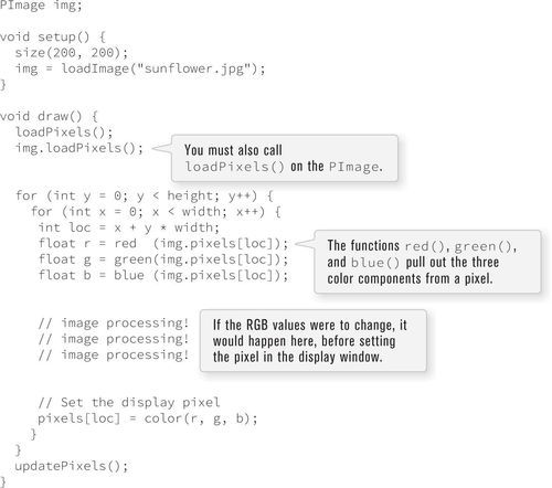
Access to these fields allows you to loop through all the pixels of an image and display them onscreen.
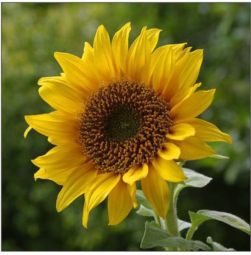
Figure 15-9
Now, you could certainly come up with simplifications in order to merely display the image (e.g., the nested loop is not required, not to mention that using the image() function would allow you to skip all this pixel work entirely). However, Example 15-7 provides a basic framework for getting the red, green, and blue values for each pixel based on its spatial orientation — (x,y) location; ultimately, this will allow you to develop more advanced image processing algorithms.
Before you move on, I should stress that this example works because the display area has the same dimensions as the source image. If this were not the case, you would simply need to have two pixel location calculations, one for the source image and one for the display area.
int imageLoc = x + y * img.width;
int displayLoc = x + y * width;
Exercise 15-7: Using Example 15-7, change the values of r, g, and b before displaying them.
15-7 A second image processing filter, making your own tint()
Just a few paragraphs ago, you were enjoying a relaxing coding session, colorizing images and adding alpha transparency with the friendly tint() method. For basic filtering, this method did the trick. The pixel by pixel method, however, will allow you to develop custom algorithms for mathematically altering the colors of an image. Consider brightness — brighter colors have higher values for their red, green, and blue components. It follows naturally that you can alter the brightness of an image by increasing or decreasing the color components of each pixel. In the next example, I will dynamically increase or decrease those values based on the mouse’s horizontal location. (Note that the next two examples include only the image processing loop itself, the rest of the code is assumed.)


Since I am altering the image on a per pixel basis, all pixels need not be treated equally. For example, I can alter the brightness of each pixel according to its distance from the mouse.
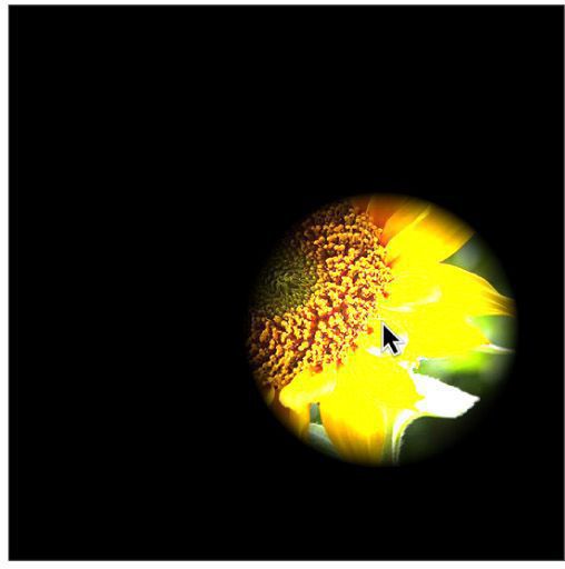
Figure 15-11

Exercise 15-8: Adjust the brightness of the red, green, and blue color components separately according to mouse interaction. For example, let mouseX control red, mouseY green, distance blue, and so on.
15-8 Writing to another PImage object’s pixels
All of the image processing examples have read every pixel from a source image and written a new pixel to the Processing window directly. However, it’s often more convenient to write the new pixels to a destination image (that you then display using the image() function). I will demonstrate this technique while looking at another simple pixel operation: threshold.
A threshold filter displays each pixel of an image in only one of two states, black or white. That state is set according to a particular threshold value. If the pixel’s brightness is greater than the threshold, I color the pixel white, less than, black. Example 15-10 uses an arbitrary threshold of 100.

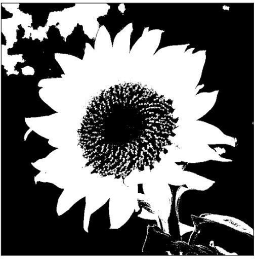
Figure 15-12
Exercise 15-9: Change the threshold according to mouseX using map().
This particular functionality is available without per pixel processing as part of Processing’s filter() function. Understanding the lower level code, however, is crucial if you want to implement your own image processing algorithms, not available with filter().
If all you want to do is threshold, Example 15-11 is much simpler.
15-9 Level II: Pixel group processing
In previous examples, you have seen a one-to-one relationship between source pixels and destination pixels. To increase an image’s brightness, you take one pixel from the source image, increase the RGB values, and display one pixel in the output window. In order to perform more advanced image processing functions, however, you must move beyond the one-to-one pixel paradigm into pixel group processing.
Let’s start by creating a new pixel out of two pixels from a source image — a pixel and its neighbor to the left.
If I know a pixel is located at (x,y):
int loc = x + y * img.width;
color pix = img.pixels[loc];
Then its left neighbor is located at (x−1,y):
int leftLoc = (x − 1) + y * img.width;
color leftPix = img.pixels[leftLoc];
I could then make a new color out of the difference between the pixel and its neighbor to the left.
float diff = abs(brightness(pix) − brightness(leftPix));
pixels[loc] = color(diff);
Example 15-12 shows the full algorithm, with the results shown in Figure 15-13.


Figure 15-13
Example 15-12 is a simple vertical edge detection algorithm. When pixels differ greatly from their neighbors, they are most likely “edge” pixels. For example, think of a picture of a white piece of paper on a black tabletop. The edges of that paper are where the colors are most different, where white meets black.
In Example 15-12, I looked at two pixels to find edges. More sophisticated algorithms, however, usually involve looking at many more neighboring pixels. After all, each pixel has eight immediate neighbors: top left, top, top right, right, bottom right, bottom, bottom left, and left. See Figure 15-14.

Figure 15-14
These image processing algorithms are often referred to as a “spatial convolution.” The process uses a weighted average of an input pixel and its neighbors to calculate an output pixel. In other words, that new pixel is a function of an area of pixels. Neighboring areas of different sizes can be employed, such as a 3 × 3 matrix, 5 × 5, and so on.
Different combinations of weights for each pixel result in various effects. For example, an image can be sharpened by subtracting the neighboring pixel values and increasing the centerpoint pixel. A blur is achieved by taking the average of all neighboring pixels. (Note that the values in the convolution matrix add up to 1.)
For example,
Sharpen:
−1 −1 −1
−1 9 −1
−1 −1 −1
Blur:
1/9 1/9 1/9
1/9 1/9 1/9
1/9 1/9 1/9
Example 15-13 performs a convolution using a 2D array (see Chapter 13 for a review of 2D arrays) to store the pixel weights of a 3 × 3 matrix. This example is probably the most advanced example you have encountered in this book so far, since it involves so many elements (nested loops, 2D arrays, pixels, etc.).
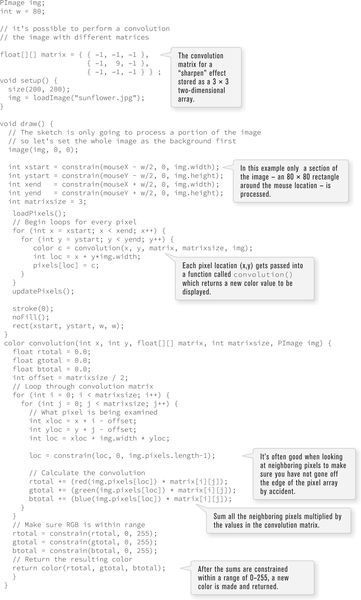

Figure 15-15
Exercise 15-10: Try different values for the convolution matrix.
Exercise 15-11: Using the framework established by the image processing examples, create a filter that takes two images as input and generates one output image. In other words, each pixel displayed should be a function of the color values from two pixels, one from one image and one from another. For example, can you write the code to blend two images together (without using tint())?
15-10 Creative visualization
You may be thinking: “Gosh, this is all very interesting, but seriously, when I want to blur an image or change its brightness, do I really need to write code? I mean, can’t I use Photoshop?” Indeed, what I have covered here is merely an introductory understanding of what highly skilled programmers at Adobe do. The power of Processing, however, is the potential for real-time, interactive graphics applications. There is no need for you to live within the confines of “pixel point” and “pixel group” processing.
Following are two examples of algorithms for drawing Processing shapes. Instead of coloring the shapes randomly or with hard-coded values as I have in the past, I am going to select colors from the pixels of a PImage object. The image itself is never displayed; rather, it serves as a database of information that you can exploit for your own creative pursuits.
In this first example, for every cycle through draw(), I will fill one ellipse at a random location onscreen with a color taken from its corresponding location in the source image. The result is a “pointillist-like” effect. See Figure 15-16.

Figure 15-16

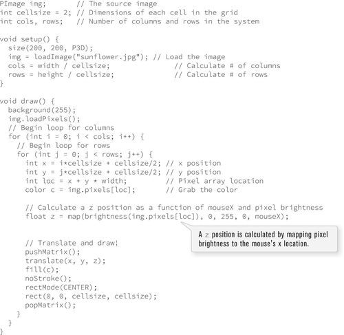
In this next example, I’ll take the data from a two-dimensional image and, using the 3D translation techniques described in Chapter 14, render a rectangle for each pixel in three-dimensional space. The z position is determined by the brightness of the color. Brighter colors appear closer to the viewer and darker ones further away.
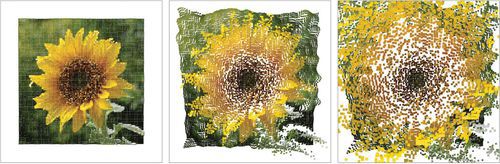
Figure 15-17
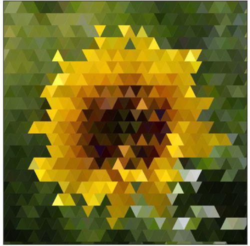
Exercise 15-12
Create a sketch that uses shapes to display a pattern that covers an entire window. Load an image and color the shapes according to the pixels of that image. The following image, for example, uses triangles.