20-1 Basic sound playback

The first thing you want to do is play a sound file in a Processing sketch. Just like with video in Processing, to be able to do anything with sound, you need the import statement at the top of your code.

import processing.sound.*;

Now that you have imported the library, you have the whole world (of sound) in your hands. I’ll start by demonstrating how to play sound from a file. Before a sound can be played, it must be loaded into memory, much in the same way images files were loaded before they could be displayed. Here, a SoundFile object is used to store a reference to a sound from a file.

SoundFile song;

The object is initialized by passing the sound filename to the constructor, along with a reference to this.

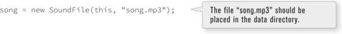
Just as with images, loading the sound file from the hard drive is a slow process so the previous line of code should be placed in setup() so as to not hamper the speed of draw().

The type of sound files compatible with Processing is limited. Possible formats are wav, aiff, and mp3. If you want to use a sound file that is not stored in a compatible format, you could download a free audio editor, such as Audacity (http://audacity.sourceforge.net/) and convert the file. Once the sound is loaded, playing is easy.

If you want your sound to loop forever, call loop() instead.

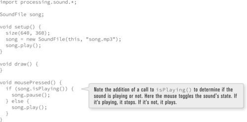
A sound can be stopped with stop() or pause(). Here is an example that plays a sound file (in this case, an approximately two-minute song) as soon as the Processing sketch begins and pauses (or restarts) the sound when the user clicks the mouse.

Example 20-1

Soundtrack

Playback of sound files is also useful for short sound effects. The following example plays a doorbell sound whenever the user clicks on the circle. The Doorbell class implements simple button functionality (rollover and click) and just happens to be a solution for Exercise 9-8 on page 180. The code for the new concepts (related to sound playback) is shown in bold type.

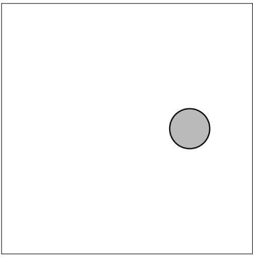
Figure 20-1

If you run the Doorbell example and click on the doorbell many times in rapid succession, you will notice that the sound restarts every time you click. It’s not given a chance to finish playing. While this is not much of an issue for this straightforward example, stopping a sound from restarting can be very important in other, more complex sound sketches. The simplest way to achieve such a result is always to check and see if a sound is playing before you call the play() function. The function isPlaying() does exactly this, returning true or false. I used this function in the previous example to determine whether the sound should be paused or played. Here, I want to play the sound if it’s not already playing, that is,

Exercise 20-2: Create a button that toggles the pause / playing state of a sound. Can you make more than one button, each tied to its own sound?

20-2 A bit fancier sound playback

During playback, a sound sample can be manipulated in real time. Volume, pitch, and pan can all be controlled.

Let’s start with volume. The technical word for volume in the world of sound is amplitude. A SoundFile object’s volume can be set with the amp() function, which takes a floating point value between 0.0 and 1.0 (0.0 being silent, 1.0 being the loudest). The following snippet assumes a file named “song.mp3” and sets its volume based on mouseX position (by mapping it to a range between 0 and 1).

Panning refers to volume of the sound in two speakers (typically a “left” and “right”). If the sound is panned all the way to the left, it will be at maximum value in the left and not heard at all in the right. Adjusting the panning in code works just as with amplitude, only the range is between −1.0 (for full pan to the left) and 1.0 (for full pan to the right).

The pitch is altered by changing the rate of playback (i.e., faster playback is higher pitch, slower playback is lower pitch) using rate(). A rate at 1.0 is normal speed, 2.0 is twice the speed, etc. The following code uses a range from 0 (where you would not hear it at all) to 4 (a rather fast playback rate).

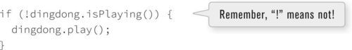
The following example adjusts the volume and pitch of a sound according to mouse movements. Note the use of loop() instead of play(), which loops the sound over and over rather than playing it one time.

Example 20-3

Sound manipulation

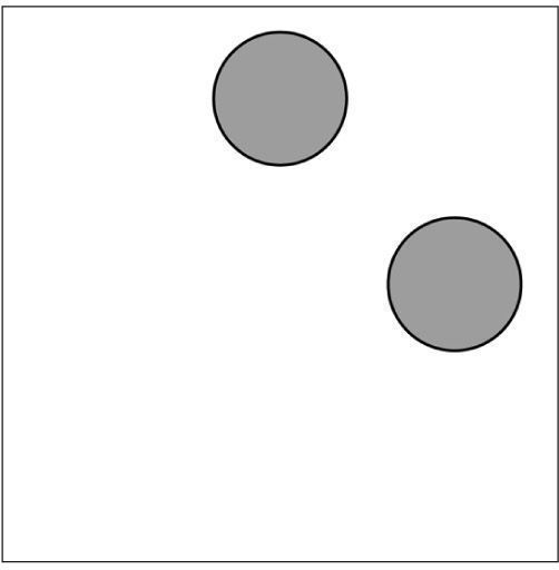
Figure 20-2

The next example uses the same sound file but pans the sound left and right.

Example 20-4

Sound manipulation

Exercise 20-3: In Example 20-3, flip the Y-axis so that the lower sound plays when the mouse is down rather than up.

Exercise 20-4: Using the bouncing ball sketch from Example 5-6, play a sound effect every time the ball bounces off a window’s edge. Pan the effect left and right according to the x-position.

Sounds can also be manipulated by processing them with an effect, such as reverb, delay feedback, and high, low, and band pass filters. These effects require the use of a separate object to process the sound. (You’ll see this same technique in more detail when I demonstrate sound analysis Section 20-4 on page 464 as well.)

A reverb filter (which occurs when a sound bounces around a room causing it to repeat, like a very fast echo) can be applied with the Reverb object.

The amount of reverb can be controlled with the room() function. Think of a room built in a way that causes more or less reverb (ranging from 0 to 1.) Here’s an example applying reverb.

Example 20-5

Reverb effect

20-3 Sound synthesis

In addition to playing sounds that load from a file, the Processing sound library has the capability of creating sound programmatically. A deep discussion of this topic is beyond the scope of this book, but I’ll introduce a few of the basic concepts. Let’s begin by thinking about the physics of sound itself. Sound travels through a medium (most commonly air, but also liquids and solids) as a wave. For example, a speaker vibrates creating a wave that ripples through the air and rather quickly arrives at your ear. You encountered the concept of a wave briefly in Section 13-10 on page 250 when I demonstrated visualizing the sin() function in Processing. In fact, sound waves can be described in terms of two key properties associated with sine waves: frequency and amplitude.

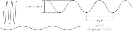
Figure 20-3

Take a look at the above diagram of waves at variable frequencies and amplitudes. The taller ones have higher amplitudes (the distance between the top and bottom of the wave) and the shorter ones lower. Amplitude is another word for volume, higher amplitudes mean louder sounds.

The frequency of a wave is related to how often it repeats (whereas the terms period and cycle refer to the inverse: how long it takes for a full cycle of the wave). A high frequency wave (or higher pitched sound) repeats often, and a lower frequency wave is stretched out and appears wider. Frequency is typically measured in hertz (Hz). One Hz is one cycle per second. Audible frequencies typically range between 20 and 20,000 Hz but what you can synthesize in Processing also highly depends on the sophistication of your speakers. In the diagram, high frequency waves are towards the top and low frequencies at the bottom.

You can specify the amplitude and frequency of a sound wave programatically in Processing with oscillator objects. An oscillation (a motion that repeats itself) is another term for wave. An oscillator that produces a sine wave is a SinOsc object.

SinOsc osc = new SinOsc(this);

If you want to hear the generated sound wave through the speakers, you can then call play().

osc.play();

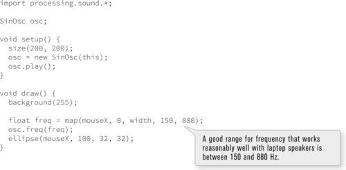
As the program runs, you can control the frequency and amplitude of the wave. Frequency is adjusted with freq() which expects a value in Hz. Adjusting the frequency has a similar effect to rate(). To adjust the volume of the oscillation, call the amp() function as you did with sound files.

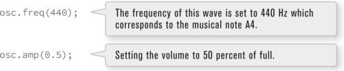
Here’s a quick example that controls the frequency of the sound with the mouse.

Example 20-6

Sound synthesis

The generated sound can also be panned from left to right (−1 to 1) using pan ().

There are also other types of waves you can generate with Processing. They include a saw wave (SawOsc), square wave (SqrOsc), triangle wave (TriOsc), and pulse wave (Pulse). While each wave has a different sound quality, they can all be manipulated with the same functions as previously described.

A more sophisticated way to simulate a musical instrument playing a note can be accomplished with an audio envelope. An envelope controls how a note begins and ends through four parameters.

1. Attack Time: this refers to the beginning of the note (like the moment you hit a key on a piano); how long it takes for the volume of the note to go from zero to its peak.

2. Sustain Time: this refers to the amount of time the note plays.

3. Sustain Level: this is the peak volume of the sound during its duration (from attack to release).

4. Release Time: this refers to the length of time it takes for the level to decay from the sustain level to zero.

To play a note with an envelope, you need both an oscillator and an envelope.

TriOsc triOsc = new TriOsc(this);

Envelope env = new Envelope(this);

To play the note, call play() on both the oscillator and the envelope. For the envelope, however, you pass in four arguments: attack time, sustain time, sustain level, and release time. The times are all floating point values specifying the number of seconds, and the level is value between 0 and 1, specifying the amplitude.

triOsc.play();

env.play(triOsc, 0.1, 1, 0.5, 1);

In the above code, the sound takes a tenth of second (0.1) to fade in to a 50 percent (0.5) amplitude, lasts for a second (1), and fades out over a second (1).

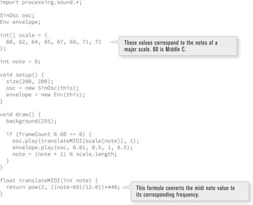
Here is an example that plays the scale from Exercise 20-5 on page 462 using an envelope. In addition, this example uses MIDI note values. MIDI stands for Musical Instrument Digital Interface and is an audio standard for communication between digital musical devices. MIDI notes can be converted into frequencies with the following formula.

$\mathit{frequency}={\left(\frac{\mathit{note}-69}{12}\right)}^2\times 440$

Example 20-7

Melody with envelope

In addition to waves, you can generate audio “noise” in Processing. In Chapter 13, I discussed distributions of random numbers and noise. In Chapter 15, I used random pixels to generate an image, and it looked a bit like static.

If you vary how a noise algorithm picks the numbers the image quality will change. Perlin noise, for example, generates a texture that looks a bit like clouds. The same can be said for audio noise. Depending on how you choose the random numbers, the result might sound harsher or smoother.

Figure 20-4

Audio noise is commonly described using colors. White noise, for example, is the term for an even distribution of random amplitudes over all frequencies. Pink noise and brown noise, however, are louder at lower frequencies and softer at higher frequences. If nothing else, the ability to generate noise in Processing may help you sleep at night. Here’s a quick example that plays white noise, controlling the volume of the noise with the mouse.

20-4 Sound analysis

In Section 19-8 on page 444, I discussed at how serial communication allows a Processing sketch to respond to input from an external hardware device connected to a sensor. Analyzing the sound from a microphone is a similar pursuit. Not only can a microphone record sound, but it can determine if the sound is loud, quiet, high-pitched, low-pitched, and so on. A Processing sketch could therefore determine if it’s running in a crowded room based on sound levels, or whether it’s listening to a soprano or bass singer based on frequency levels. This section will cover how to use a sound’s amplitude and frequency data in a sketch.

Let’s begin by building a very simple example that ties the size of a circle to the volume level. To do this you first need to create an Amplitude object. This object’s sole purpose in life is to listen to a sound and report back its amplitude (i.e., volume).

Amplitude analyzer = new Amplitude(this);

Once you have the Amplitude object, you next need to connect sound that you want to analyze. This is accomplished with the input() function. This works similarly to how I plugged a SoundFile into the Reverb object in Example 20-3. The following code loads a sound file and passes it to an analyzer. But, as you’ll see in a moment, you can apply this technique to any type of sound, including input from a microphone.

SoundFile song = new SoundFile(this, “song.mp3”);

analyzer.input(song);

To retrieve the volume, you then call analyze() which will return an amplitude value between 0 and 1.

float level = analyzer.analyze();

Here is all of the above put together in a single example, using the sound file from Example 20-3. The sound level controls the size of an ellipse. The new parts are bolded.

To read the volume from a microphone, you need to plug a different input into the Amplitude object. To accomplish this, create an AudioIn object and call start() to begin the process of listening to the microphone.

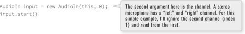
If for any reason you want to hear the microphone input come out of your speakers, you can also say input.play(). In this case, I don’t want to cause audio feedback so I’m leaving that out. Putting it all together, I can now recreate Example 20-9 with live input.

Example 20-9

Amplitude analysis

Exercise 20-6: Rewrite Example 20-10 with left and right volume levels mapped to different circles.

Example 20-10

Live Microphone Input

20-5 Sound thresholding

A common sound interaction is triggering an event when a sound occurs. Consider “the clapper.” Clap, the lights go on. Clap again, the lights go off. A clap can be thought of as a very loud and short sound. To program “the clapper” in Processing, I’ll need to listen for volume and instigate an event when the volume is high.

In the case of clapping, you might decide that when the overall volume is greater than 0.5, the user is clapping (this is not a scientific measurement, but is good enough for now). This value of 0.5 is known as the threshold. Above the threshold, events are triggered, below, they are not.

float volume = analyzer.analyze();

if (volume > 0.5) {

 // DO SOMETHING WHEN THE VOLUME IS GREATER THAN ONE!

}

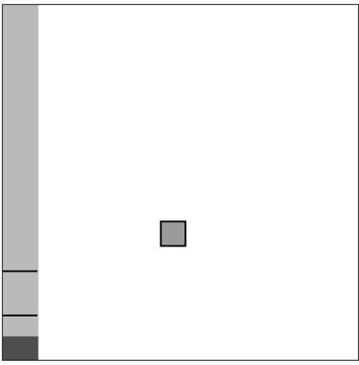
Example 20-11 draws rectangles in the window whenever the overall volume level is greater than 0.5. The volume level is also displayed on the left-hand side as a bar.

Example 20-11

Sound threshold

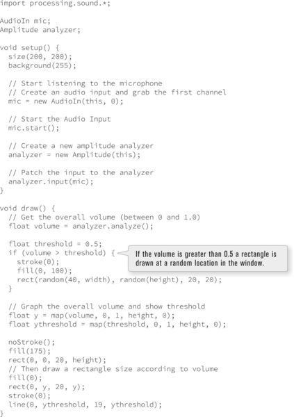
Figure 20-5

This application works fairly well, but does not truly emulate the clapper. Notice how each clap results in several rectangles drawn to the window. This is because the sound, although seemingly instantaneous to human ears, occurs over a period of time. It may be a very short period of time, but it’s enough to sustain a volume level over 0.5 for several cycles through draw().

In order to have a clap trigger an event one and only one time, I’ll need to rethink the logic of this program. In plain English, this is what I’m trying to achieve:

• If the sound level is above 0.5, then you are clapping and trigger the event. However, do not trigger the event if you just did a moment ago!

The key here is how you define “a moment ago.” One solution would be to implement a timer, that is, only trigger the event once and then wait one second before you are allowed to trigger the event again. This is a perfectly OK solution. Nonetheless, with sound, a timer is totally unnecessary since the sound itself will tell you when you have finished clapping!

• If the sound level is less than 0.25, then it is quiet and you have finished clapping.

OK, with these two pieces of logic, you are ready to program this “double-thresholded” algorithm. There are two thresholds, one to determine if you have started clapping, and one to determine if you have finished. You will need a boolean variable to tell you whether you are currently clapping or not.

Assume clapping equals false to start.

• If the sound level is above 0.5, and you are not already clapping, trigger the event and set clapping = true.

• If you are clapping and the sound level is less than 0.25, then it is quiet and set clapping = false.

In code, this translates to:

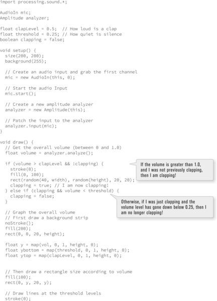
// If the volume is greater than one, and I am not clapping, draw a rectangle

if (vol > 0.5 && !clapping) {

 // Trigger event!

 clapping = true; // I am now clapping!

} else if (clapping && vol < 0.25) { // If I am finished clapping

 clapping = false;

}

Here is the full example where one and only one rectangle appears per clap.

Figure 20-6

Example 20-12

Sound events (double threshold)

Exercise 20-8: Create a simple game that is controlled with volume. Suggestion: First make the game work with the mouse, then replace the mouse with live input. Some examples are Pong, where the paddle’s position is tied to volume, or a simple jumping game, where a character jumps each time you clap.

20-6 Spectrum analysis

Analyzing the volume of a sound in Processing is only the beginning of sound analysis. For more advanced applications, you might want to know the volume of a sound at various frequencies? Is this a high-frequency or a low-frequency sound?

The process of spectrum analysis takes a sound signal (a wave) and decodes it into a series of frequency bands. You can think of these bands like the “resolution” of the analysis. With many bands you can more precisely pinpoint the amplitude of a given frequency. With fewer bands, you are looking for the volume of a sound over a wider range of frequencies.

To do this analysis, you first need an FFT object. The FFT object serves the same purpose as the previous example’s Amplitude. This time, however, it will provide an array of amplitude values (one for each band) rather than a single overall volume level. FFT stands for “Fast Fourier Transform” (named for the French mathematician Joseph Fourier) and refers to the algorithm that transforms the waveform to an array of frequency amplitudes.

FFT fft = new FFT(this, 512);

Notice how the FFT constructor requires a second argument: an integer. This value specifies the number of frequency bands in the spectrum you want to produce; a good default is 512 but it can really be any number you want. One band, incidentally, is the equivalent ofjust making an Amplitude analyzer object.

The next step, just as with amplitude, is to plug in the audio (whether from a file, generated sound, or microphone) into the FFT object.

SoundFile song = new SoundFile(this, “song.mp3”);

fft.input(song);

Again, just as with amplitude, the next step is to call analyze().

fft.analyze();

Here, though, I am simply telling the analyzer to run the FFT algorithm. To look at the actual results, I have to examine the FFT object’s spectrum array. This array holds the amplitude values (between 0 and 1) for all of the frequency bands. The length of the array is equal to the number of bands requested in the FFT constructor (512 in this case). I can loop through this array, as follows:

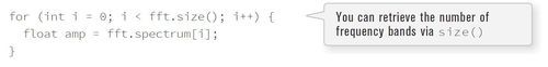
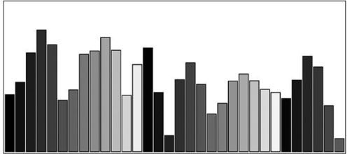
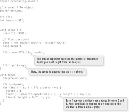
Here is all the above code put together into an example. It draws each frequency band as a line with height tied to the particular amplitude of that frequency.

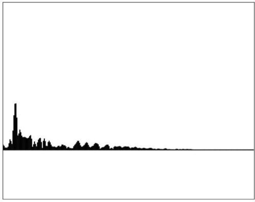
Figure 20-7

Example 20-13

Spectrum analysis

Exercise 20-9: Perform the same spectrum analysis of a signal from microphone input.

Exercise 20-10

Using a smaller number of bands, create a visualization of the spectrum with a “graphic equalizer” look. See the image below for an example.