
Translation and Rotation (in 3D!)
In this chapter:
– Using P3D and P2D renderers
– Vertex shapes
– 2D and 3D rotation
– Saving and restoring the transformation state: pushMatrix() and popMatrix()
14-1 The z-axis
As you have seen throughout this book, pixels in a two-dimensional window are described using Cartesian coordinates: an x (horizontal) and a y (vertical) position. This concept dates all the way back to Chapter 1, when I discussed thinking of the screen as a digital piece of graph paper.
In three-dimensional space (such as the actual, real-world space where you’re reading this book), a third axis (commonly referred to as the z-axis) refers to the depth of any given point. In a Processing sketch’s window, a coordinate along this z-axis indicates how far in front or behind the window a pixel lives. Scratching your head is a perfectly reasonable response here. After all, a computer window is only two dimensional. There are no pixels floating in the air in front of or behind your LCD monitor! In this chapter, I will examine how using the theoretical z-axis will create the illusion of three-dimensional space in your Processing window.
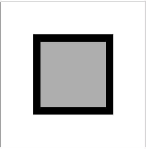
I can, in fact, create a three-dimensional illusion with what you have learned so far. For example, if I were to draw a rectangle in the middle of the window and slowly increase its width and height, it might appear as if it’s moving toward the viewer. See Example 14-1.
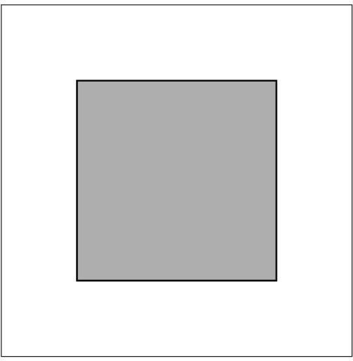
Figure 14-1
Is this rectangle flying off of the computer screen about to bump into your nose? Technically, this is, of course, not the case. It’s simply a rectangle growing in size. But I have created the illusion of the rectangle moving toward you.
Fortunately, if you choose to use 3D coordinates, Processing will create the illusion for you. While the idea of a third dimension on a flat computer monitor may seem imaginary, it is quite real for Processing. Processing knows about perspective, and selects the appropriate two-dimensional pixels in order to create the three-dimensional effect. You should recognize, however, that as soon as you enter the world of 3D pixel coordinates, a certain amount of control must be relinquished to the Processing renderer. You can no longer control exact pixel locations as you might with 2D shapes, because (x,y) locations will be adjusted to account for 3D perspective.
In order to specify points in three dimensions, the coordinates are specified in the order you would expect: (x,y,z). Cartesian 3D systems can be described as left-handed or right-handed. If you use your right hand to point your index finger in the positive y-direction (up) and your thumb in the positive x direction (to the right), the rest of your fingers will point toward the positive z direction. It’s left-handed if you use your left hand and do the same. In Processing, the system is left-handed, as shown in Figure 14-2.

Figure 14-2
My first goal is to rewrite Example 14-1 using the 3D capabilities of Processing. Assume the following variables:
int x = width/2;
int y = height/2;
int z = 0;
int r = 10;
In order to specify the location for a rectangle, the rect() function takes four arguments: x location, y location, width, and height.
rect(x, y, w, h);
Your first instinct might be to add another argument to the rect() function.
The Processing reference page for rect(), however, does not allow for this possibility. In order to specify 3D coordinates for shapes in the Processing world, you must learn to use a new function, called translate().
The translate() function is not exclusive to 3D sketches, so let’s return to two dimensions to see how it works.
The function translate() moves the origin point — (0,0) — relative to its previous state. When a sketch first starts, the origin point lives on the top left of the window. If you were to call the function translate() with the arguments (50,50), the result would be as shown in Figure 14-3.

Figure 14-3
You can think of it as moving a pen around the screen, where the pen indicates the origin point.
In addition, the origin always resets itself back to the top left corner at the beginning of draw(). Any calls to translate() only apply to the current cycle through the draw() loop. See Example 14-2.

Figure 14-4
Now that I’ve discussed how translate() works, I can return to the original problem of specifying 3D coordinates. translate(), unlike rect(), ellipse(), and other shape functions, can accept a third argument for a z position.

The above code translates 50 units along the z-axis, and then draws a rectangle at (100,100). While the above is technically correct, when using translate(), it’s a good habit to specify the (x,y) location as part of the translation, that is:

Finally, I can use a variable for the z position and animate the shape moving toward the viewer, as seen in Example 14-3.

Although the result does not look different from Example 14-1, it’s quite different conceptually as I have opened the door to creating a variety of three-dimensional effects on the screen with Processing’s 3D engine.
Exercise 14-1
Fill in the appropriate translated() functions to create this pattern. Once you’re finished, try adding a third argument to translate() to move the pattern into three dimensions.

size(200, 200);
background(0);
stroke(255);
fill(255, 100);
translate(___________, ___________);
rect(0, 0, 100, 100);
translate(___________, ___________);
rect(0, 0, 100, 100);
translate(___________, ___________);
line(0, 0, −50, 50);
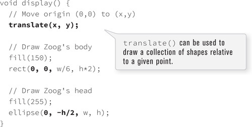
The translate() function is particularly useful when you’re drawing a collection of shapes relative to a given centerpoint. Harking back to Zoog from the first 10 chapters of this book, you saw code like this:
// Draw Zoog’s body
fill(150);
rect(x, y, w/6, h*2);
// Draw Zoog’s head
fill(255);
ellipse(x, y−h/2, w, h);
}
The display() function above draws all of Zoog’s parts (body and head, etc.) relative to Zoog’s (x,y) location. It requires that x and y be used in both rect() and ellipse(). translate() allows me to simply set Processing’s origin (0,0) at Zoog’s (x,y) location and therefore draw the shapes relative to (0,0).
14-2 What is P3D exactly?
If you look closely at Example 14-3, you will notice that I have added a third argument to the size() function. Traditionally, size() has served one purpose: to specify the width and height of a Processing window. The size() function, however, also accepts a third parameter indicating a drawing mode or “renderer”. The renderer tells Processing what to do behind the scenes when rendering the display window. The default renderer (when none is specified) employs existing Java 2D libraries to draw shapes, set colors, and so on. You do not have to worry about how this works. The creators of Processing took care of the details.
If you want to employ 3D translation (or rotation as you will see later in this chapter), the default renderer will no longer suffice. Running the example results in the following error:
“translate(), or this particular variation of it, is not available with this renderer.”
Instead of switching back translate(x, y), you’ll want to select a different renderer: P3D. P3D is a 3D renderer that employs hardware acceleration. If you have an OpenGL compatible graphics card installed on your computer (which is pretty much every computer), you can use this renderer. P3D also often has an added advantage: speed. If you are planning to display large numbers of shapes onscreen in a high-resolution window, this mode will likely have the best performance. There is also a P2D renderer for the case where you would like the features of OpenGL but are drawing 2D graphics.
To specify the rendering mode, add a third argument in all caps to the size() function.
size(200, 200); // using the default renderer
size(200, 200, P3D); // using P3D
size(200, 200, P2D); // using P2D
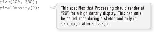
Finally, in the case of high “pixel density” displays (for example, an Apple “Retina” display), Processing can also render at “2X” with pixelDensity(). Pixel density is different than pixel resolution which is defined as the actual width and height of an image in pixels. A high density display is measured in DPI (“dots per inch”). Density here refers to how many pixels (i.e., dots) fit into each physical inch of your display. For high density displays, Processing offers renderers that double the number of pixels to make shapes appear finer to the human eye. This all happens behind the scenes and you don’t need to change the values in your code — the width and height of your sketch remain the same. However, some complications are introduced when working with direct access to pixels which I’ll briefly discuss in the next chapter.
Exercise 14-2: Run any Processing sketch in the default renderer, then switch to P2D and P3D. Notice any difference?
14-3 Vertex shapes
Up until now, your ability to draw to the screen has been limited to a small list of primitive two-dimensional shapes: rectangles, ellipses, triangles, lines, and points. For some projects, however, creating your own custom shapes is desirable. This can be done through the use of the functions beginShape(), endShape(), and vertex().
Consider a rectangle. A rectangle in Processing is defined as a reference point, as well as a width and height.
rect(50, 50, 100, 100);
But you could also consider a rectangle to be a polygon (a closed shape bounded by line segments) made up of four points. The points of a polygon are called vertices (plural) or vertex (singular). The following code draws exactly the same shape as the rect() function by setting the vertices of the rectangle individually. See Figure 14-5.
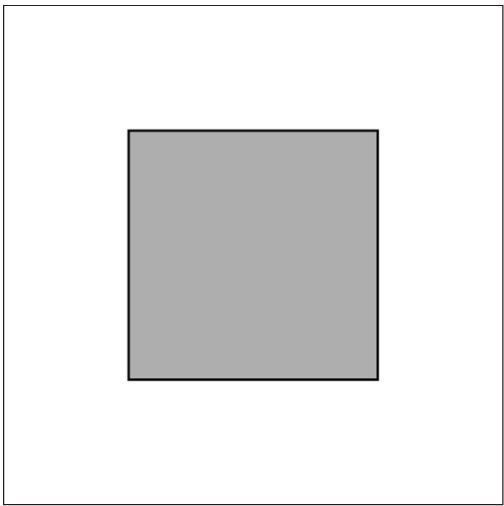
Figure 14-5
vertex(50, 50);
vertex(150, 50);
vertex(150, 150);
vertex(50, 150);
endShape(CLOSE);
beginShape() indicates that you are going to create a custom shape made up of some number of vertex points: a single polygon. vertex() specifies the points for each vertex in the polygon and endShape() indicates that you are finished adding vertices. The argument CLOSE inside of endShape(CLOSE) declares that the shape should be closed, that is, that the last vertex point should connect to the first.
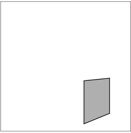
The nice thing about using a custom shape over a simple rectangle is flexibility. For example, the sides are not required to be perpendicular. See Figure 14-6.
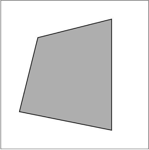
Figure 14-6
stroke(0);
fill(175);
beginShape();
vertex(50, 50);
vertex(150, 25);
vertex(150, 175);
vertex(25, 150);
endShape(CLOSE);
You also have the option of creating more than one shape, for example, in a loop, as shown in Figure 14-7.

Figure 14-7
stroke(0);
for (int i = 0; i < 10; i++) {
beginShape();
fill(175);
vertex(i*20, 10 − i);
vertex(i*20 + 15, 10 + i);
vertex(i*20 + 15, 180 + i);
vertex(i*20, 180−i);
endShape(CLOSE);
}
You can also add an argument to beginShape() specifying exactly what type of shape you want to make. This is particularly useful if you want to make more than one polygon. For example, if you create six vertex points, there is no way for Processing to know that you really want to draw two triangles (as opposed to one hexagon) unless you say beginShape(TRIANGLES). If you do not want to make a polygon at all, but want to draw points or lines, you can by saying beginShape(POINTS) or beginShape(LINES). See Figure 14-8.

Figure 14-8
beginShape(LINES);
for (int i = 10; i < width; i += 20) {
vertex(i, 10);
vertex(i, height−10);
}
endShape();
Note that LINES is meant for drawing a series of individual lines, not a continous loop. For a continuous loop, do not use any argument. Instead, simply specify all the vertex points you need and include noFill(). See Figure 14-9.
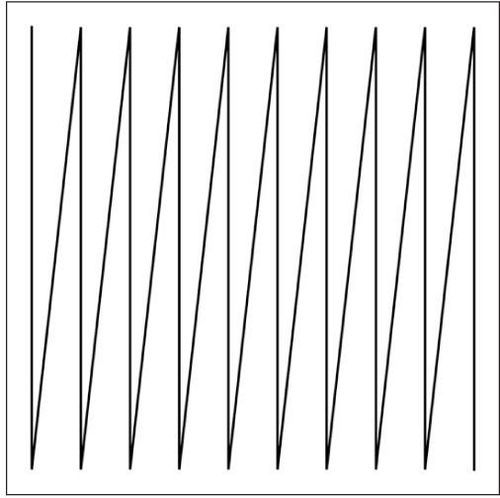
Figure 14-9
noFill();
stroke(0);
beginShape();
for (int i = 10; i < width; i += 20) {
vertex(i, 10);
vertex(i, height − 10);
}
endShape();
The full list of possible arguments for beginShape() is available in the Processing reference (http://processing.org/reference/beginShape_.html): POINTS, LINES, TRIANGLES, TRIANGLE_FAN, TRIANGLE_STRIP,QUADS, and QUAD_STRIP.
In addition, vertex() can be replaced with curveVertex() to join the points with curves instead of straight lines. With curveVertex(), note how the first and last points are not displayed. This is because they are required to define the curvature of the line as it begins at the second point and ends at the second to last point. See Figure 14-10.
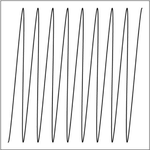
Figure 14-10
noFill();
stroke(0);
beginShape();
for (int i = 10; i < width; i +=20) {
curveVertex(i, 10);
curveVertex(i, height − 10);
}
endShape();
Exercise 14-3
Complete the vertices for the shape pictured.
size(200, 200);
background(255);
stroke(0);
fill(175);
beginShape();
vertex(20, 20);
vertex(____________, ____________);
vertex(____________, ____________);
vertex(____________, ____________);
vertex(____________, ____________);
endShape(____________);

14-4 Custom 3D shapes
Three-dimensional shapes can be created using beginShape(), endShape(), and vertex() by placing multiple polygons side by side in the proper configuration. Let’s say you want to draw a four-sided pyramid made up of four triangles, all connected to one point (the apex) and a flat plane (the base). If the shape is simple enough, you might be able to get by with just writing out the code. In most cases, however, it’s best to start sketching it out with pencil and paper to determine the location of all the vertices. One example for a pyramid is shown in Figure 14-11.

Figure 14-11
Example 14-4 takes the vertices from Figure 14-11 and puts them in a function that allows the pyramid to be drawn at any size. (As an exercise, try making the pyramid into an object.)
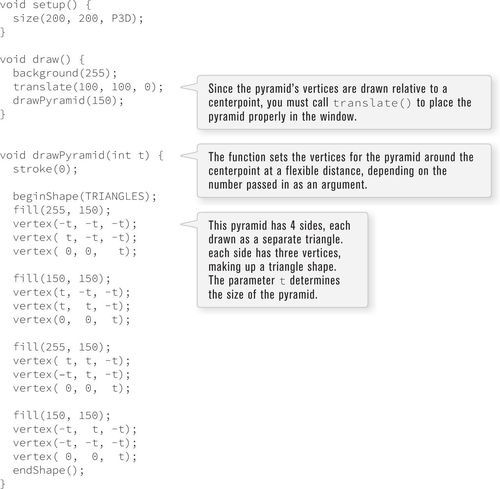

Figure 14-12
Exercise 14-4: Create a pyramid with only three sides. Include the base (for a total of four triangles). Use the space below to sketch out the vertex locations as in Figure 14-11.
Exercise 14-5: Create a three-dimensional cube using eight quads — beginShape(QUADS). (Note that a simpler way to make a cube in Processing is with the box() function.)
14-5 Simple rotation
There is nothing particularly three-dimensional about the visual result of the pyramid example. The image looks more like a flat rectangle with two lines connected diagonally from end to end. Again, you have to remind yourself that I am only creating a three-dimensional illusion, and it’s not a particularly effective one without animating the pyramid structure within the virtual space. One way for me to demonstrate the difference would be to rotate the pyramid. So let’s learn about rotation.
For most people, in the physical world, rotation is a pretty simple and intuitive concept. Grab a baton, twirl it, and you have a sense of what it means to rotate an object.
Programming rotation, unfortunately, is not so simple. All sorts of questions come up. Around what axis should you rotate? At what angle? Around what origin point? Processing offers several functions related to rotation, which I will explore slowly, step by step. My goal will be to program a solar system simulation with multiple planets rotating around a star at different rates (as well as to rotate the pyramid in order to better experience its three dimensionality).
But first, let’s try something simple and attempt to rotate one rectangle around its center. I should be able to get rotation going with the following three principles:
1. Shapes are rotated in Processing with the rotate() function.
2. The rotate() function takes one argument, an angle measured in radians.
3. rotate() will rotate the shape in the clockwise direction (to the right).
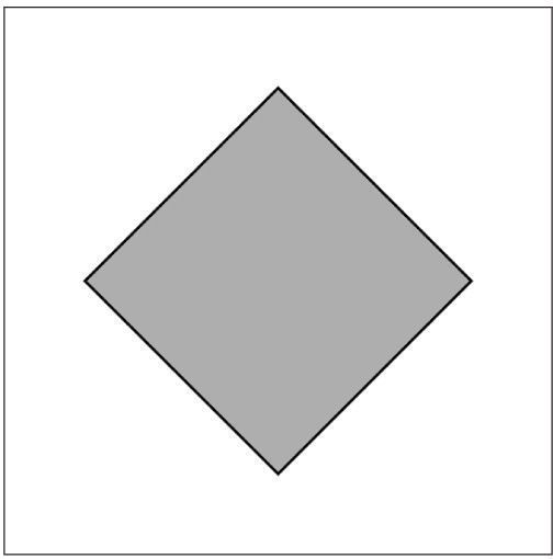
OK, armed with this knowledge, I should be able to just call the rotate() function and pass in an angle. Say, 45° (or PI/4 radians) in Processing. Here is a first (albeit flawed) attempt, with the output shown in Figure 14-13.
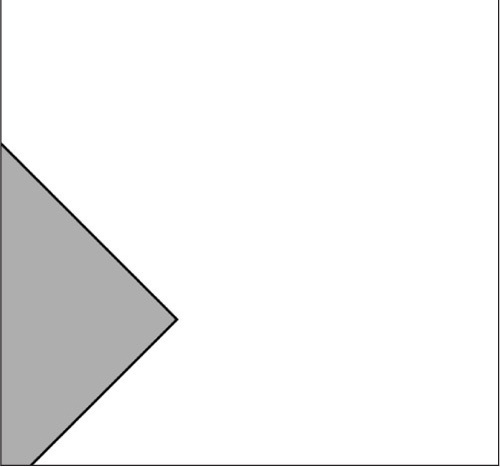
Figure 14-13
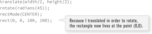
rectMode(CENTER);
rect(width/2, height/2, 100, 100);
Shoot. What went wrong? The rectangle looks rotated, but it’s in the wrong place!
The single most important fact to remember about rotation in Processing is that shapes always rotate around the point of origin. Where is the point of origin in this example? The top left corner! The origin has not been translated. The rectangle therefore will not spin around its own center. Instead, it rotates around the top left corner. See Figure 14-14.
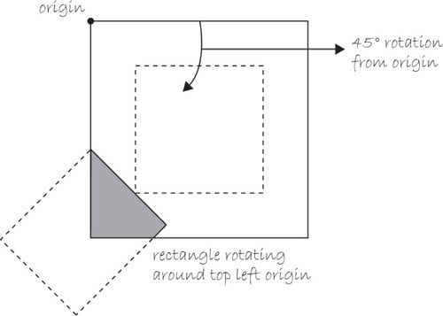
Figure 14-14
Sure, there may come a day when all you want to do is rotate shapes around the top left corner, but until that day comes, you will always need to first move the origin to the proper location before rotating, and then display the rectangle. translate() to the rescue!
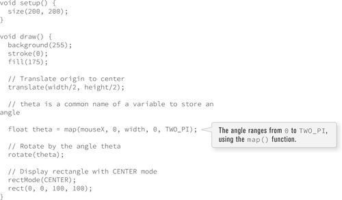
I can expand the above code using the mouseX location to calculate an angle of rotation and thus animate the rectangle, allowing it to spin. See Example 14-5.

14-6 Rotation around different axes
Now that I have basic rotation out of the way, you can ask the next important rotation question:
Around which axis do I want to rotate?
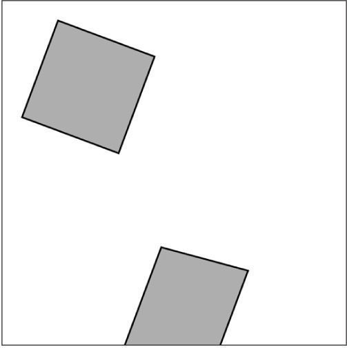
In the previous section, the square rotated around the z-axis. This is the default axis for two-dimensional rotation. See Figure 14-16.
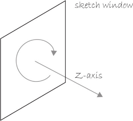
Figure 14-16
Processing also allows for rotation around the x or y-axis with the functions rotateX() and rotateY(), which each require the P3D renderer. The function rotateZ() also exists and is the equivalent of rotate(). See Example 14-6, Example 14-7 and Example 14-8.

Figure 14-19
The rotate functions can also be used in combination. The results of Example 14-9 are shown in Figure 14-20.
Figure 14-20
Returning to the pyramid example, you will see how rotating makes the three-dimensional quality of the shape more apparent. The example is also expanded to include a second pyramid that is offset from the first pyramid using translate. Note, however, that it rotates around the same origin point as the first pyramid (since rotateX() and rotateY() are called before the second translate()).


Exercise 14-7: Rotate the 3D cube you made in Exercise 14-5 on page 277. Can you rotate it around the corner or center? You can also use the Processing function box() to make the cube.
Exercise 14-8: Make a Pyramid class.
14-7 Scale
In addition to translate() and rotate(), there is one more function, scale(), that affects the way shapes are oriented and drawn onscreen. scale() increases or decreases the size of objects onscreen. Just as with rotate(), the scaling effect is performed relative to the origin’s location.
scale() takes a floating point value, a percentage at which to scale: 1.0 is 100%. For example, scale(0.5) draws an object at 50% of its size and scale(3.0) increases the object’s size to 300%.
Following is a re-creation of Example 14-1 (the growing square) using scale().
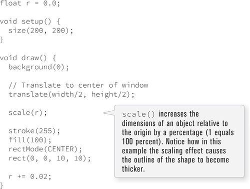
scale() can also take two arguments (for scaling along the x and y axes with different values) or three arguments (for the x, y, and z axes).
14-8 The matrix: pushing and popping
What is the matrix?
In order to keep track of rotations and translations and how to display the shapes according to different transformations, Processing (and just about any computer graphics software) uses a matrix.
How matrix transformations work is beyond the scope of this book; however, it’s useful to simply know that the information related to the coordinate system is stored in what is known as a transformation matrix. When a translation or rotation is applied, the transformation matrix changes. From time to time, it’s useful to save the current state of the matrix to be restored later. This will ultimately allow you to move and rotate individual shapes without them affecting others.
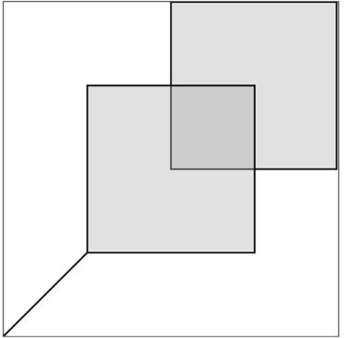
This concept is best illustrated with an example. Let’s give ourselves an assignment: Create a Processing sketch where two rectangles rotate at different speeds in different directions around their respective center points.
As I start developing this example, you will see where the problems arise and how I’ll need to utilize the functions pushMatrix() and popMatrix().
Starting with essentially the same code from Section 14-4 on page 275, I can rotate a square around the z-axis in the top left corner of the window. See Example 14-12.

Figure 14-23
Making some minor adjustments, let’s now implement a rotating square in the bottom right-hand corner.
Without careful consideration, I might think to simply combine the two programs. The setup() function should stay the same, I should incorporate two global variables, theta1 and theta2, and call the appropriate translation and rotation for each rectangle. I should also adjust translation for the second square from translate(150, 150); to translate(100, 100);, since I’ve already translated to (50,50) with the first square. This should work, right?
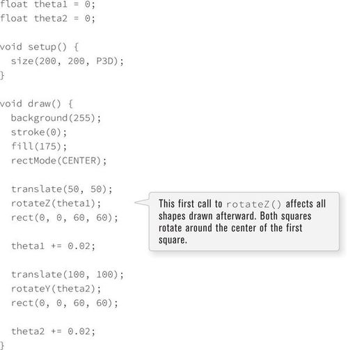
Running this example quickly reveals a problem. The first (top left) square rotates around its center. However, while the second square does rotate around its center, it also rotates around the first square! Remember, all calls to translate and rotate are relative to the coordinate system’s previous state. I need a way to restore the matrix to its original state so that individual shapes can act independently.
Saving and restoring the rotation/translation state is accomplished with the functions pushMatrix() and popMatrix(). To get started, let’s think of them as saveMatrix() and restoreMatrix(). (Note there are no such functions.) Push = save. Pop = restore.
For each square to rotate on its own, I can write the following algorithm (with the new parts bolded).
1. Save the current transformation matrix. This is where I started, with (0,0) in the top left corner of the window and no rotation.
2. Translate and rotate the first rectangle.
3. Display the first rectangle.
4. Restore matrix from Step 1 so that the second rectangle isn’t affected by Steps 2 and 3!
5. Translate and rotate the second rectangle.
6. Display the second rectangle.
Rewriting the code in Example 14-14 gives the correct result as shown in Figure 14-26.
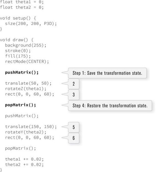
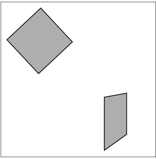
Figure 14-26
Although technically not required, it’s a good habit to place pushMatrix() and popMatrix() around the second rectangle as well (in case I was to add more to this code). A nice rule of thumb when starting is to use pushMatrix() and popMatrix() before and after translation and rotation for all shapes so that they can be treated as individual entities. In fact, this example should really be object oriented, with every object making its own calls to pushMatrix(), translate(), rotate(), and popMatrix(). See Example 14-15.
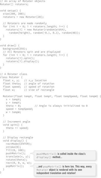
Figure 14-27
Interesting results can also be produced from nesting multiple calls to pushMatrix() and popMatrix(). There must always be an equal number of calls to both pushMatrix() and popMatrix(), but they do not always have to come one right after the other.
To understand how this works, let’s take a closer look at the meaning of “push” and “pop.” “Push” and “pop” refer to a concept in computer science known as a stack. Knowledge of how a stack works will help you use pushMatrix() and popMatrix() properly.
A stack is exactly that: a stack. Consider an English teacher getting settled in for a night of grading papers stored in a pile on a desk, a stack of papers. The teacher piles them up one by one and reads them in reverse order of the pile. The first paper placed on the stack is the last one read. The last paper added is the first one read. Note this is the exact opposite of a queue. If you’re waiting in line to buy tickets to a movie, the first person in line is the first person to get to buy tickets, the last person is the last. See Figure 14-28.
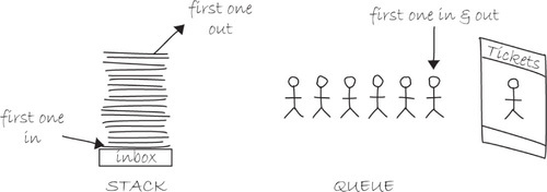
Figure 14-28
Pushing refers to the process of putting something in the stack, popping to taking something out. This is why you must always have an equal number of pushMatrix() and popMatrix() calls. You can’t pop something if it does not exist! If your numbers are off, an error will appear in the console. For example, with too many calls to popMatrix(), Processing will report: “Missing a pushMatrix() to go along with that popMatrix().”
Using the rotating squares program as a foundation, you can hopefully see how nesting pushMatrix() and popMatrix() is useful. The following sketch has one circle in the center (let’s call it the sun) with another circle rotating it (let’s call it earth) and another two rotating around it (let’s call them moon #1 and moon #2).
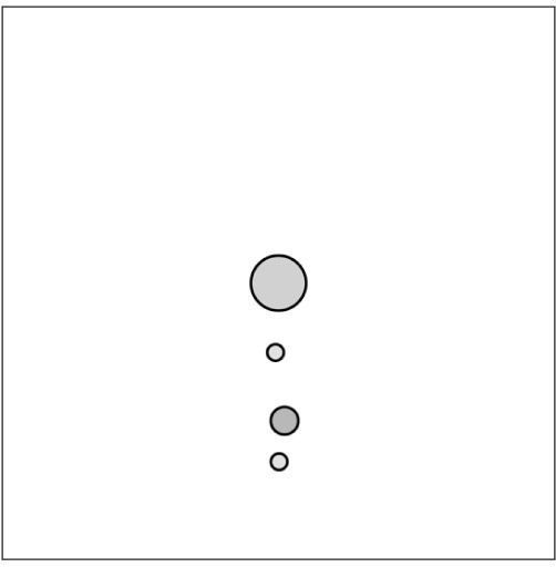
Figure 14-29
pushMatrix() and popMatrix() can also be nested inside for or while loops with rather unique and interesting results. The following example is a bit of a brainteaser, but I encourage you to play around with it.

Exercise 14-9: Take either your pyramid or your cube shape and make it into a class. Have each object make its own call to pushMatrix() and popMatrix(). Can you make an array of objects all rotating independently in 3D?
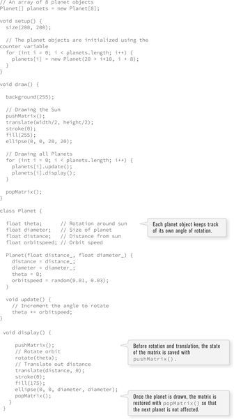
14-9 A Processing solar system
Using all the translation, rotation, pushing, and popping techniques in this chapter, you are ready to build a Processing solar system. This example is an updated version of Example 14-16 in the previous section (without any moons), with two major changes:
• Every planet is an object, a member of a Planet class.
• An array of planets orbits the sun.


Exercise 14-10: How would you add moons to the planets? Hint: Write a Moon class that is virtually identical to the Planet one. Then, incorporate a Moon variable into the Planet class. (In Chapter22, I will show how this could be made more efficient with advanced OOP techniques.)
Exercise 14-11: Extend the solar system example into three dimensions. Try using sphere() or box() instead of ellipse(). Note sphere() takes one argument, the sphere’s radius. box() can take one argument (size, in the case of a cube) or three arguments (width, height, and depth.)
14-10 PShape
At the very beginning of this book, the first thing you learned is how to draw “primitive” shapes to the screen: rectangles, ellipses, lines, triangles, and more. You’ve now seen in this chapter a more advanced drawing option using beginShape() and endShape() to specify the vertices of a custom polygon in both two and three dimensions.
This is all well and good and will get you pretty far. There’s very little you can’t draw just knowing the above. However, there is another step. A step that can, in some cases, improve the speed of your rendering as well as offer a more advanced organizational model for your code — PShape().
By now, you are hopefully quite comfortable with the idea of data types. You specify them often — a float variable called speed, an int named x, perhaps even a char entitled letterGrade. These are all primitive data types, bits sitting in the computer’s memory ready for your use. Though perhaps a bit trickier, you are also beginning to feel at ease with objects, complex data types that store multiple pieces of data (along with functionality) — the Zoog class, for example, included floating point variables for location, size, and speed as well as methods to move, display itself, and so on. Zoog, of course, is a user-defined class; I brought Zoog into this programming world, defined what it means to be a Zoog, and defined the data and functions associated with a Zoog object.
In addition to user-defined objects, Processing has a bunch of built-in classes for you to use. The next chapter will be entirely dedicated to one of these built-in Processing objects: PImage, a class for loading and displaying images.
Before I move onto the next chapter, let’s wade into the waters by examining PShape, a datatype for storing shapes. A PShape can store custom geometry you build via an algorithm as well as shapes that you load from an external file, such as a scalable vector graphics files (SVG), a standard file format for storing shape data.
A PShape object can be created with either the createShape function or loadShape(), in the case of loading from a file. Let’s take a look at a quick example, a more thorough discussion of PShape, beyond the scope of this book, is included at the Processing tutorials page (https://processing.org/tutorials/pshape/)

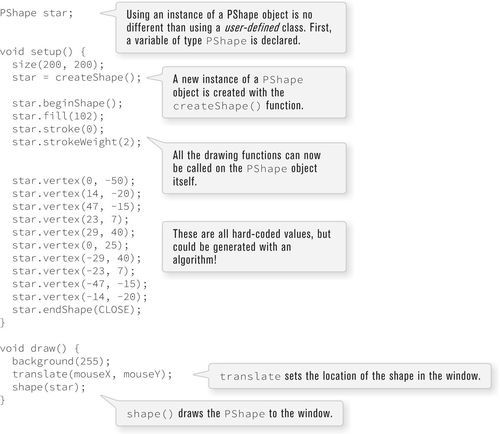
Exercise 14-12
Rewrite Example 14-19 so that the PShape object itself is inside your own Star class that also includes x,y variables for position. Make multiple instances of the object an array. Here is some code to get you started.
class Star {
// The PShape object
PShape s;
// The location where I will draw the shape
float x, y;
Star() {
// What goes here?
}
void move() {
// What goes here?
}
void display() {
// What goes here?
}
}
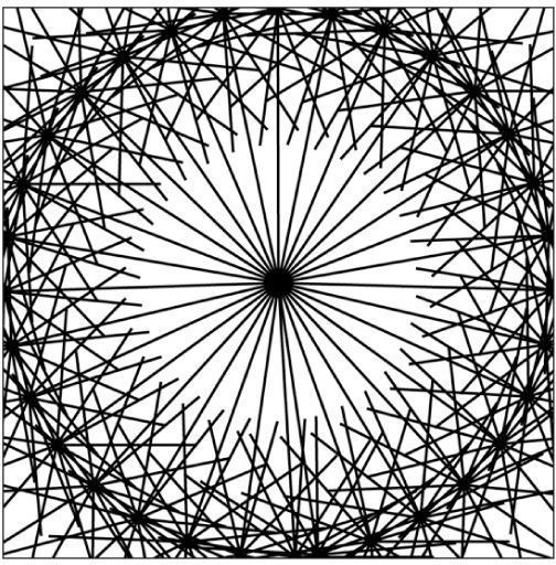
Lesson Six Project
Create a virtual ecosystem. Make a class for each “creature” in your world. Using the techniques from Chapters 13 and 14, attempt to infuse your creatures with personality. Some possibilities:
• Use Perlin noise to control the movements of creatures.
• Make the creatures look like they are breathing with oscillation.
• Design the creatures using recursion.
• Design the custom polygons using beginShape().
• Use rotation in the creatures’ behaviors.
Use the space provided below to sketch designs, notes, and pseudocode for your project.