
Chapter 12. Network Function Virtualization
Chapter 11—which is dedicated to Network Virtualization Overlays (NVO)—described a modern paradigm for the integration of virtual machines (VMs), containers, and bare-metal servers in a (private, public, or telco) cloud. The resulting overlay provides connectivity between subscribers and VMs, or between different VMs. The latter are typically servers, which behave like IP endpoints. Subscribers also behave like IP endpoints, therefore a typical service example would be a TCP session between a subscriber client and a VM acting as a database server (or a web server) in the cloud.
Network Function Virtualization (NFV) takes advantage of NVO by allowing VMs (or containers) to actually perform a network service function. These VMs are typically in-line and instead of acting as communication endpoints, they are transit devices, with a left and a right interface. There are many examples of such network service functions: stateful firewalling, Network Address Translation (NAT), load balancing, Distributed Denial-of-Service (DDoS) detection and mitigation, Deep Packet Inspection (DPI), Intrusion Detection and Prevention (IDS/IDP), IPSec/TLS tunnel termination, proxy functions, and so on.
Note
Throughout this chapter, every time you see the term VM, you can think of either a VM or a container. Network functions can be implemented on any of these virtual compute entities (and on physical devices, too).
Depending on the actual service provided by the Virtual Network Function (VNF), a VM may act as follows:
- As an IP endpoint
- For example, a VM can establish TCP sessions, becoming a TCP client or server for both left-facing and right-facing sessions. An archetypical use case is a web proxy. From a network architecture perspective, this model is similar to a plain NVO in which the VM has two interfaces—one left-facing and one right-facing. The NVO does not need to perform any fancy traffic steering, because the IP endpoints are at the VM itself.
- As a transit element in the IP communications
- In this case, the VM acts upon packets, and the IP endpoints are outside the VM. For example, a TCP session might transit this VM in such a way that the VM is neither the client nor the server of that session. This is a genuine network function and it’s the main focus of this chapter.
NFV in the Software-Defined Networking Era
NFV was initially proposed as a paradigm to implement network functions over Intel x86–based architectures. Its natural applicability to cloud infrastructures makes NFV interesting, attractive, and timely. Before diving into the details, let’s step back for a moment and analyze NFV from a broader business perspective.
A first motivation for NFV is the perceived ability to reduce capital expenditures (CAPEX), assuming that x86-based commodity servers can be cheaper than vendor-specific hardware and application-specific integrated circuits (ASICs). And they are. Commodity servers are much cheaper than, for example, a router, by quite a substantial factor. But that is comparing apples to oranges because the biggest source of cost in our industry is software development, not hardware or hardware development. If there are no hardware sales to amortize the software R&D, software needs to be priced based on its development costs, and summed up to the x86 commodity servers. In addition to the various software components, there’s also the operating system (OS), the virtualization layer, and the orchestration layer, which all come with any new NFV components or elements.
Virtual or Physical?
Anyway, let’s take the software costs out of the discussion and imagine a hypothetical world where all the network service applications were open source, supported, and reliable. Does NFV replace the need for physical network devices? Not always. It all depends on the actual requirements. Let’s answer this question after a brief technical introduction.
In the NFV world, the term virtual is used somewhat in a misleading manner. For many people, something is virtual if it is executed in general-purpose processors based on the Intel x86 architecture. This is actually a very narrow definition. This book is full of virtual things; for example, VPNs are virtual, but they are orthogonal to x86.
Software is ubiquitous and is not only restricted to general-purpose processors. For example, network device ASICs typically execute microcode. Although this microcode used to be very limited in the past, in recent years it has dramatically increased in flexibility and richness. One good example is Juniper’s Trio architecture, whose microcode programmability makes it possible to implement any new encapsulation with software.
Table 12-1 provides a comparison between the three available platforms to execute network function software.
| Function flexibility | Network performance | Power efficiency | Platform portability | |
|---|---|---|---|---|
| Intel x86 | High | Low | Low | High |
| Custom Silicon | High | High | High | Mediuma |
| Merchant Silicon | Low | High | Medium | Low |
a *For both Junos and IOS XR, the control plane has always run on general-purpose processors. However, until very recently the low-level microcode instructions that execute on custom ASICs were not portable to x86. With Juniper virtual MX—and soon Cisco virtual ASR—a fully x86-compatible OS emulates both the control-plane and the forwarding-engine ASICs. In this way, the software that runs on custom silicon is portable to x86. | ||||
Note
Faithful ASIC emulations over x86 typically have a lower performance for two reasons: the interplatform adaptation layers, and the intrinsic limitations of the x86 architecture. There is no free lunch.
Intel x86 processors
The x86 architecture is specialized for complex computation tasks and provides the best environment in which to program, test, and deploy new applications. That is where it excels over any other technology. But, because it is general purpose, it can perform many functions and not all at the same level of efficiency. Packet-forwarding functions do not require complex computation steps (with the exception of encryption/decryption) but instead need fast context switching and memory lookup. The key aspect for efficiency when it comes to packet forwarding is the ability to parallelize. Certainly x86 can do packet forwarding, but at the expense of efficiency, and that (if you are looking for scale) means higher power consumption, higher space, higher cooling requirements, and ultimately, potentially higher total cost of ownership (TCO).
The barriers preventing the Intel x86 architecture from achieving better forwarding performance are well known: clock frequency limits, challenges to increase number of cores, chipset size constraints, number of pins, and so on. All these constraints have set a slow pace of incremental improvement. Unless something very innovative is discovered, the ability to substantially grow packet-forwarding capacity for Intel x86 CPUs is questionable.
Intel x86 remains a great platform for many use cases. Indeed, if the required packet-processing performance is low, Intel x86 is the best way to go. As mentioned earlier, several networking vendors have virtual—or rather, x86-adapted—images of their network OSs. And the possibility of deploying new innovative services on x86 is bound only by the imagination.
Custom ASICs
Custom ASICs are designed by networking vendors and have the richest and most flexible packet plus flow-processing features. If the target packet-processing performance is medium or high while the processing logic required is somewhat complex, custom silicon provides the lowest TCO—despite having a higher cost per unit.
Merchant ASICs
Merchant ASICs are designed and produced by chip vendors. Networking vendors write the software for the ASICs and ship them in self-branded network devices. As a result, the very same ASIC may be present in the equipment sold by different vendors. These chips typically have a very efficient pipeline, which is adapted to simple straight-line code, but as soon as the code has branching and looping—as is typically required for the sophisticated features in the network edge—these ASICs are neither efficient nor even capable of fulfilling the functionality requirements.
The bottom line is that there are several available architectures to execute network software functions, and they are all valid but not equivalent. Each has its own pros. The network designer must carefully choose among the options for each use case.
Applicability of NFV to Service Providers
After the technical foundations are laid, let’s pursue the market analysis. Traffic growth on networks is still at 40%–50%, or even more, year on year. The network capacity required to sustain such demand growth must be at least at that level. The only way for the ecosystem to be sustainable is to have the following capacity growth characteristics:
-
It is larger than the demand growth.
-
It is at the same or lower cost, because demand growth does not necessarily drive revenue growth.
Such capacity growth is ultimately sustained on edge routers, core routers, security systems, and switching systems that increase their forwarding density at such pace. This hardware also keeps improving its footprint in terms of space, power consumption, cooling requirements, and so on.
As for the x86 architecture, it improves its packet-forwarding capacity on average 10% per year. A generalized shift of the networking industry toward NFV would lead to a capacity growth below the demand growth. Such a difference would need to be paid in number of units deployed, with the associated increase in CAPEX and OPEX.
Taking all of these factors into account, NFV has its best use case on the low-traffic regime. Does it make it irrelevant? No, not at all. NFV is a key enabler of network agility. If there is any single challenge that service providers (SPs) face, it is agility: introducing new services and new capabilities on their infrastructure, changing network behavior, and ultimately, reacting faster and with lower costs to new requirements. In one sentence: quickly adapting to the present and future demands of the market. And with traffic growth at 40%–50% year on year, there’s a strong business reason why network agility is more important than ever.
Traditionally, the ISP business model has focused on large-scale services such as residential or mobile access, assuming that statistical gain drives the economics into the green zone. But these services are now commoditized: the revenue associated with them has already reached a plateau, if not decreased due to competition. Being able to provide new services in an agile manner is paramount.
On the other hand, shifting from a business model with one single service for ten million subscribers to another with one thousand services—and ten thousand subscribers for each service—is a major challenge. What if the service does not attain market traction? And if the validation cycle is so long that the service is already obsolete by the time it is finally launched?
Here is where NFV comes into play. The key factor is uncertainty. The more uncertainty there is about a service or about the demand, the more convenient it will be to approach it with NFV. And the more certainty there is about a service or demand (expected number of subscribers, traffic patterns, etc.), the more suitable a hardware technology will be.
Any new service or new function deployed on the network, mainly at the edge, starts with a lot of uncertainty. It is hard to predict how much traffic it will consume, how many subscribers are needed for the service to be profitable, how successful it will be, how fast the demand will grow, and so on. It is at this stage where an NFV-based deployment provides agility, lower entry costs, and a faster time to market. As demand grows, stabilizes, or becomes more predictable, uncertainties transform into knowledge. Then, cost efficiency per service unit likely becomes a priority, and only ASICs offer the capacity required to address the next phases of the service deployment.
On the other hand, NFV can play a major role in trying out new services with the guarantee that you can shut it down without a major upfront investment. In conclusion, NFV is a key tool for SPs to address many new small opportunities, each one characterized by a high uncertainty.
So, it’s not a black-and-white decision between going virtual or going physical. Both have key roles at different phases of network growth and viability. They can definitely coexist on a network infrastructure, be connected to one another, and with the right tools also be seamlessly operated. This is what we go on to discuss in this chapter: how VNFs can be interconnected (chained) using technologies, such as MPLS, that can be naturally extended to hardware elements. In short, MPLS in the SDN era!
NFV Practical Use Case
Figure 12-1 shows a common NFV use case that will serve as this chapter’s reference example. In it, subscribers access the Internet through a Service Function Chain (SFC)—frequently just called Service Chain—that consists of three VMs: SI_A, SI_B, and SI_C. The acronym SI stands for service instance, and here it is basically a VM that performs a network function. Being a VM, the function is virtualized by definition, so it is an NFV.
Each service instance performs a different network function and these are executed in sequence. For the moment, let’s assume that none of these functions is NAT. In other words, the original IP source and destination addresses are maintained throughout the entire packet life—represented in Figure 12-1 as a snake-like double-arrowed solid line.
Similar to the NVO chapter and for exactly the same reasons, the examples in this NFV chapter are based on OpenContrail and the main challenge is finding a way to steer the traffic through the entire service function chain.
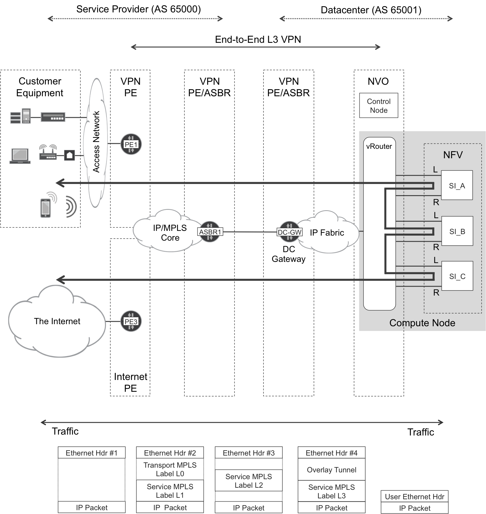
Figure 12-1. SFC inserted in an Internet access
Note
NFV is typically intersubnet. For simplicity, let’s assume that the Virtual Networks (VNs) are in L3 mode.
Let’s get into the heart of NFV and its forwarding and control planes.
NFV Forwarding Plane
As compared to its control plane, NFV’s forwarding plane is quite simple, because it is just a combination of features that have already been described in this book. The signaling and forwarding in Figure 12-2 should look familiar if you have thoroughly read all the previous chapters.
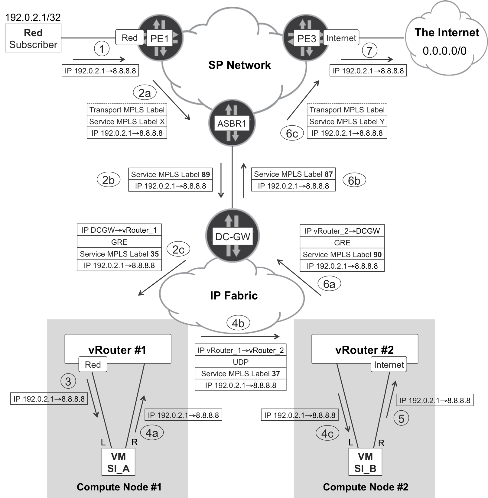
Figure 12-2. NFV—forwarding plane
Let’s review a short description of the signaling.
PE3 injects the 0/0 prefix into the VPN Internet. This route is propagated in IP VPN format via BGP, reaching the NVO control nodes—not shown in the picture—after several session hops. Control nodes convey this information to the vRouter agents via XMPP. Then, some magic route leaking takes place inside the NVO; as a result, the control nodes advertise the same 0/0 route into VPN Red, up to the data center gateway (DC-GW). This advertisement reaches PE1 after several BGP session hops.
Note
This chapter focuses on left-to-right or subscriber-to-Internet traffic. The reverse path is strictly symmetrical—with reversed source and destination IP addresses, and different MPLS labels. The subscriber’s address 192.0.2.1 is reachable from VPN Internet through the NVO and, finally, VPN Red.
Figure 12-2 also illustrates a service chain with two service instances (for simplicity, the external one-hop L2 headers are not shown). Although it is perfectly possible to run both service instances on the same compute node, this example features them in different compute nodes in order to again illustrate the overlay connection between vRouters.
Here is the sequence for left-to-right packets that go from the subscriber to the Internet (note that the number sequence is also represented in Figure 12-2):
-
The Red subscriber, as a CE, sends a plain IP packet to PE1.
-
This part of the forwarding path takes place in the context of IP VPN Red. PE1 and vRouter_1 are the ingress and egress PE, respectively. PE1 processes the packet in VRF Red—strictly speaking, the VRF name is Red:Red. The MPLS service label changes twice, once at each of the Option B ASBRs (ASBR1 and DC-GW), which perform a next-hop-self operation on the BGP control plane.
-
vRouter_1, as an egress IP VPN PE, pops the MPLS service label. This label is associated to a CE: the VM interface (vNIC) connected to the left interface of VM SI_A.
-
The magic of the service function chain takes place and the remainder of the chapter unveils the magic. For the moment, just note that inside each vRouter the packet is plain IP, whereas it requires an overlay encapsulation to jump between vRouters.
-
The VM SI_B acts like a CE and sends the packet out of its right interface.
-
This next part of the forwarding path takes place in the context of IP VPN Internet. vRouter_2 and PE3 are the ingress and egress PEs, respectively. vRouter_2 processes the packet in the context of VRF Internet—strictly speaking, the VRF name is Internet:Internet. The MPLS service label changes twice, once at each of the Option B ASBRs (DC-GW and ASBR1), which perform a next-hop-self operation on the BGP control plane. As discussed in Chapter 3, it is possible to establish eBGP sessions from a VRF to connect to the Internet.
-
Finally, PE3 pops the last MPLS label and sends the packet out to the Internet.
There are several missing pieces in the puzzle, like the packet processing and forwarding inside the service instance VMs, or the service-chain implementation.
Regarding the VMs, let’s assume for the moment that they implement interface-based forwarding: if a VM receives a packet on the left interface and the packet is not dropped (and it is not destined for the VM itself), the VM sends it out of the right interface. Conversely, what arrives on the right is forwarded out of the left interface. This topic is discussed at the end of this chapter.
Let’s now focus on how OpenContrail builds the service chain by linking the service instances, and how the traffic is steered through the chain.
NFV—VRF Layout Models
Let’s review sequence 4a in Figure 12-2. When the packet arrives to vRouter_1 from SI_A’s right interface, it must be processed in the context of a VRF. But, which one?
-
If it is VRF Red:Red, the next hop would be the vNIC connected to the left interface of VM SI_A. This would create a forwarding loop, so it is not an option.
-
If it is VRF Internet:Internet, the next hop would be the DC-GW and the packet would escape the service chain without being processed by VM SI_B. Again, this is not an option.
So, this reasoning highlights that more auxiliary VRFs are needed to instantiate a service function chain.
If you look back at Figure 3-5, service chaining is not a new concept; in fact, it has existed for decades in SP networks. However, that asymmetrical route target (RT) chaining strategy is not particularly efficient—especially for long chains—and it is not easy to automate and operate.
OpenContrail supports the two alternative mechanisms to build SFCs depicted in Figure 12-3 and listed here:
-
The transit VN model, referenced in draft-fm-bess-service-chaining as “Service Function Instances Connected by Virtual Networks”.
-
The two-VN model, referenced in draft-fm-bess-service-chaining as “Logical Service Functions Connected in a Chain”
Although not explicitly shown in this particular figure, you can definitely distribute service instances across different compute nodes.
Note
Remember that OpenContrail allows creating VNs, whereas VRFs are automatically instantiated from VNs. By default, VN Red is linked to one single VRF called Red:Red.
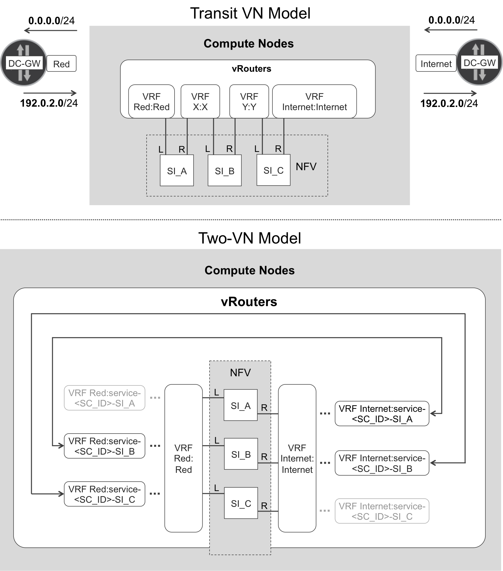
Figure 12-3. Two Service Function Chain models
Legacy VRF Layout—Transit VN Model
This legacy model requires N-1 transit VNs (named X and Y in Figure 12-3) for an SFC consisting of N service instances. The only purpose of these transit VNs is to build the chain. Although the following statement is not strictly accurate, you can view this model as functionally based on a 1:1 VN:VRF mapping. It is worthwhile to quickly review this model because it establishes a valuable conceptual foundation that you will need to understand other paradigms.
Transit VN model—configuration
Here are the steps to configure an SFC with transit VRFs using OpenContrail GUI—there are equivalent methods using the CLI and the north-bound API, too:
-
At Configure→Networking→Networks, define the entry-exit VNs, namely Red and Internet. Each of these VNs requires an RT that matches on the corresponding VRF at the gateway nodes. Assign at least one subnet to each VN for vNIC address allocation.
-
At Configure→Networking→Networks, define the transit VNs, namely X and Y. These VNs are flagged Allowed Transit and, because they are not propagated to gateway nodes, they do not need any RTs explicitly configured. Assign at least one subnet to each VN for vNIC address allocation.
-
At Configure→Services→Service Templates, define one template for each different network function. Typically, for a three-instance chain you need three templates. These specify the VM image to use and the interfaces that it will have. Typically, you need left, right, and management interfaces—the latter is not shown in the figures, because it does not participate on the SFC. (You can read more about templates at the end of this chapter.)
-
At Configure→Services→Service Instances, launch SI_A, SI_B, and SI_C from their corresponding templates. Place the left and right interfaces of each instance into the appropriate VN according to the upper part of Figure 12-3. Note that unlike regular VMs, which are defined at the compute controller, network service VMs or instances are defined at the NVO controller (OpenContrail), which in turn talks to the compute controller for the VM instantiation.
-
At Configure→Networking→Policies, define three policies. The first one should specify that traffic between VN Red and VN X should go through service SI_A. The second one should specify that traffic between VN X and VN Y should go through service SI_B. And the third policy should specify that traffic between VN Y and VN Internet should go through service SI_C.
-
At Configure→Networking→Networks, assign the previously created policies to the appropriate networks: first policy to VN Red and VN X; second policy to VN X and VN Y; and, third policy to VN Y and VN Internet.
This policy assignment automatically leaks the routes between the VNs, taking care of next hops in order to achieve the desired traffic steering.
Transit VN model—routes and next hops
Let’s keep our focus on the top of Figure 12-3. Taking left-to-right (upstream) traffic as an example, the leaking process for the default 0/0 route goes as follows:
-
OpenContrail learns the 0/0 route from DC-GW and installs it on VRF Internet:Internet, setting DC-GW as the (MPLS-labeled) next hop.
-
OpenContrail leaks the 0/0 route into VRF Y:Y, setting the next hop to the left (L) interface of VM SI_C.
-
OpenContrail leaks the 0/0 route into VRF X:X, setting the next hop to the left (L) interface of VM SI_B.
-
OpenContrail leaks the 0/0 route into VRF Red:Red, setting the next hop to the left (L) interface of VM SI_A.
-
OpenContrail advertises the 0/0 route to the DC-GW in the context of VRF Red:Red, setting the vRouter—at the compute node where SI_A is running—as the (labeled) next hop.
A similar (reverse) mechanism applies to right-to-left (downstream) traffic. It relies on left-to-right leaking of the 192.0.2.0/24 prefix, setting the right-facing interfaces of the service instance VMs as the next hops throughout the chain.
Note
NFV relies on the BGP and XMPP mechanisms already discussed in the NVO chapter. At this point, it is assumed that you know how routes are learned, advertised, and programmed in OpenContrail.
Modern VRF Layout—Two-VN Model
Let’s make a first interpretation of the center-down area of Figure 12-3. In a nutshell, VRF Red:Red has a default route 0/0 that points to the left interface of SI_A. After receiving a packet on its left interface, SI_A performs interface-based forwarding and sends the packet out of its right interface. The vRouter receives the packet from SI_A’s right interface and forwards it according to VRF Internet:service-<SC_ID>_SI_A, which is linked to VRF Red:service-<SC_ID>_SI_B, whose default route points to the left interface of SI_B. In this way, the packet flows through the chain until it exits SI_C’s right interface. At this point, the vRouter forwards the packet according to the VRF Internet:Internet table, which has a default route pointing to the outside world (DC-GW).
This alternative and modern approach for defining an SFC in OpenContrail simply relies on just two VNs: the left VN and the right VN. It will take several pages to fully describe this model so that we can make sense of it. Keep reading.
Of course, as many VNs as you like can play the left or right VN role; but within a given SFC, there is only one VN pair [left, right]. In this example, these are VNs Red and Internet, respectively. The left interface of all of the service instances are assigned to the left VN on the vRouter. Likewise, all the right interfaces are assigned to the right VN.
Let’s begin with the configuration details because they will cement the foundation to understand the actual implementation.
Two-VN model—configuration
Here are the steps to configure an SFC with transit VRFs in OpenContrail’s GUI—there are equivalent methods using the CLI and the north-bound API:
-
At Configure→Networking→Networks, define the entry-exit VNs, namely Red and Internet. Each of these VNs requires an RT that matches on the corresponding VRF at the gateway nodes. Assign at least one subnet to each VN for vNIC address allocation. No transit VNs need to be defined.
-
At Configure→Services→Service Templates, define one template for each different network function.
-
At Configure→Services→Service Instances, launch SI_A, SI_B, and SI_C from their corresponding templates. Place the left and right interfaces of each instance into the appropriate VN: left on Red, right on Internet.
-
At Configure→Networking→Policies, define one single policy. The policy states that traffic between VN Red and VN Internet should go through the following service instances in sequence: SI_A, SI_B, and SI_C.
-
At Configure→Networking→Networks, assign the previously created policy to VN Red and VN Internet.
This policy assignment automatically leaks the routes between the VNs, taking care of next hops so as to achieve the desired traffic steering. This model has a much simpler configuration scheme, given that you don’t need to define transit VNs. The complex magic happens behind the curtains.
In L3VPN terms, this magic is a combination of the following three features implemented at the vRouter (this list is dedicated to those readers who come from the SP routing and MPLS worlds—if this is not the case for you, feel free to skip it):
-
Interface leaking between VRFs so that different VRFs can resolve routes toward the same vRouter-VM interface.
-
Per-CE MPLS labels so that packets arriving from the overlay are MPLS-switched (by executing a pop operation) toward a VM, without an IPv4 lookup.
-
Filter-based forwarding (FBF), formerly known as policy-based routing (PBR), so that packets arriving from a VM are steered to a different next hop from the one dictated by the normal routing path.
Note
Here’s what mapping label X to a vRouter-VM interface means: if a packet is received with MPLS label X from an overlay tunnel, pop the label and then send the packet out of that vRouter-VM interface.
Two-VN model—routes and next hops
The two-VN model relies on a 1:N VN:VRF relationship. The administrator only creates two VNs, but these are cloned in several VRFs with different content. For example, the Red VN is linked to four VRFs—Red:Red, Red:service-<SC_ID>_SI_A, Red:service-<SC_ID>_SI_B, and Red:service-<SC_ID>_SI_C. Out of these, three are especially relevant for this chain, whereas the leftmost one is grayed-out in Figure 12-3. It could become relevant if the SFC is further extended through an additional service instance to the left.
Taking left-to-right traffic as an example (in Figure 12-3, it goes up→down), the 0/0 default route has the following next hops in the relevant VRFs at the NVO:
-
At VRF Internet:Internet, the (labeled) next hop is DC-GW.
-
At VRFs Red:service-<SC_ID>_SI_C and Internet:service-<SC_ID>_SI_B, which are linked together, the next hop is the left interface of SI_C.
-
At VRFs Red:service-<SC_ID>_SI_B and Internet:service-<SC_ID>_SI_A, which are linked together, the next hop is the left interface of SI_B.
-
At VRF Red:Red, the next hop is the left interface of SI_A.
Note
The two-VN model will be used for the remainder of this chapter. If you don’t fully understand it yet, that’s normal. Keep reading.
NFV—Long Version of the Life of a Packet
For simplicity, let’s move back to a scenario with just two service instances in the chain, rather than three. And for completeness, let’s place the two service instances at two different compute nodes. You might remember that Figure 12-2 was followed by a list of steps describing the life of a left-to-right packet, and that step 4 in that list began with a mysterious note: the magic of the service function chain takes place.
It’s time to unveil the magic. This is the life of a packet inside the SFC as illustrated in Figure 12-4:
-
The packet arrives to vRouter_1 as MPLS-over-GRE with label 35. This label corresponds to PE-CE interface tapX, so vRouter_1 pops the label and sends the packet to the left interface of VM SI_A. There is no IP lookup in this step.
-
VM SI_A performs per-interface forwarding and, after processing the packet, sends it out of its right interface. The remote endpoint of this internal link is interface tapY.
-
Although tapY belongs to VRF Internet:Internet, OpenContrail dynamically applies a VRF mapping table to the interface. This table basically says: if the incoming packet’s source IP address is VM SI_A’s right interface (10.3.3.111), map the packet to VRF Internet:Internet; otherwise, it is supposed to be a transit packet for VM SI_A, so map it to Internet:service-<SC_ID>_SI_A. The <SC_ID> field is a service chain identifier dynamically generated by the control node. In routing terms, this is FBF (or PBR).
-
VRF Internet:service-<SC_ID>_SI_A at vRouter_1 has a 0/0 route whose next hop is vRouter_2, MPLS-over-UDP, label 37.
-
The packet arrives to vRouter_2 with MPLS label 37. This label corresponds to PE-CE interface tapZ, so vRouter_2 pops the label and sends the packet to the left interface of VM SI_B. There is no IP lookup in this step.
-
VM SI_B performs per-interface forwarding, and after processing the packet, sends it out of its right interface. The remote endpoint of this internal link is interface tapT.
-
Interface tapT belongs to VRF Internet:Internet, and being the rightmost end of the SFC, there is no policy-based routing. The route in that VRF is honored and vRouter_2 sends the packet to DC-GW with MPLS service label 90. After that, it’s IP VPN with Inter-AS Option B business as usual (see Figure 12-2).
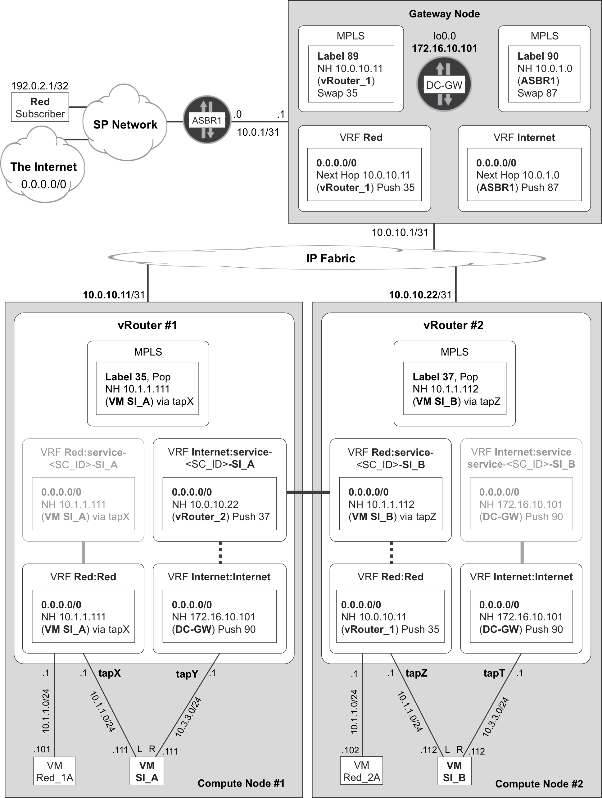
Figure 12-4. NFV routing state for left-to-right traffic
In this example, the following tables at the NVO are relevant to forwarding: MPLS table at vRouter_1, VRF Internet:service-<SC_ID>_SI_A at vRouter_1, MPLS table at vRouter_2 and VRF Internet:Internet at vRouter_2.
How about the other tables shown in Figure 12-4? They are relevant for other flows:
-
A packet traveling from the Internet to the Red subscriber is processed by: MPLS table at vRouter_2, VRF Red:service-<SC_ID>_SI_B at vRouter_2, MPLS table at vRouter_1, and VRF Red:Red at vRouter_1. Of course, the relevant route is 192.0.2.0/24 or 192.0.2.1/32—not 0/0—and the MPLS labels are different.
-
VRF Red:Red at vRouter_1 is relevant for packets sourced from VM Red_1A.
Note
Look back at the center-down area of Figure 12-3. This illustration should be easier to understand now.
NFV Control Plane
After reading Chapter 11, programming and signaling routes on the NVO should no longer be a mystery. Control nodes implement all the logic and signal it conveniently via BGP or XMPP, depending on whether the peer is a gateway node or a vRouter.
On the other hand, there are a few new logical constructs specific to NFV, like service templates, service chains, Access Control Lists (ACLs), VRF mapping tables, or links between routing instances. To illustrate this, Example 12-1 shows how the control node instructs a vRouter to assign a VRF mapping table to a tap interface.
Example 12-1. XMPP—VRF mapping table on a VM interface
1     <?xml version="1.0"?>
2     <iq type="set" from="network-control@contrailsystems.com"
3         to="default-global-system-config:vrouter_1/config">
4      <config>
5       <update>
6        <node type="virtual-machine-interface">
7         <name>default-domain:mpls-in-the-sdn-era:default-domain
8               mpls-in-sdn-era__SI_A__right__2</name>
9         <vrf-assign-table>
10         <vrf-assign-rule>
11          <match-condition>
12           <src-address>
13            <subnet>
14             <ip-prefix>10.3.3.111</ip-prefix>
15             <ip-prefix-len>32</ip-prefix-len>
16            </subnet>
17           </src-address>
18          </match-condition>
19          <routing-instance>default-domain:mpls-in-the-sdn-era:
20                            Internet:Internet</routing-instance>
21         </vrf-assign-rule>
22         <vrf-assign-rule>
23          <match-condition></match-condition>
24          <routing-instance>default-domain:mpls-in-the-sdn-era:
25                           Internet:service-71b49d3d-b710-477a-9fb9-
26                           5bc571579cfb-default-domain_mpls-in-the-
27                           sdn-era_SI_A</routing-instance>
28         </vrf-assign-rule>
29        </vrf-assign-table>
30       </node>
31      </update>
32     </config>
33    </iq>
You can see the SI_A__right__2 interface (line 8) is nothing but the right interface of VM SI_A. The numeral 2 comes from the fact that it is the right interface (left interface is 1). As for the VRF mapping table, it is applied at the vRouter side—in other words, on the interface tapY in Figure 12-4. This table applies to packets received by the vRouter from the VM.
The long identifier 71b49d3d-b710-477a-9fb9-5bc571579cfb (lines 24 and 25) is nothing but the dynamically generated service chain identifier or <SC_ID>.
The construct in Example 12-1 is the cornerstone of traffic steering through the chain. VRF Internet:Internet is only relevant for packets that are originated from SI_A. All the packets that traverse SI_A (like those going from the subscriber to the Internet) are processed in the context of VRF Internet:service-<SC_ID>_SI_A. This FBF (or PBR) mechanism is essential for the SFC to work as expected.
If, instead, a transit packet entering vRouter_1 at tapY was assigned to VRF Internet:Internet, it would exit the SFC prematurely and go to the DC-GW without being processed by SI_B.
Example 12-2 shows another interesting XMPP construct: a link between routing instances.
Example 12-2. XMPP—Link between routing instances
<?xml version="1.0"?>
<iq type="set" from="network-control@contrailsystems.com"
    to="default-global-system-config:vrouter_1/config">
 <config>
  <update>
   <link>
    <node type="routing-instance">
     <name>default-domain:mpls-in-the-sdn-era:Internet:service-
           71b49d3d-b710-477a-9fb9-5bc571579cfb-default-domain_
           mpls-in-the-sdn-era_SI_A</name>
    </node>
    <node type="routing-instance">
     <name>default-domain:mpls-in-the-sdn-era:Red:service-
           71b49d3d-b710-477a-9fb9-5bc571579cfb-default-domain_
           mpls-in-the-sdn-era_SI_B</name>
    </node>
    <metadata type="connection" />
   </link>
  </update>
 </config>
</iq>
The full signaling involved in SFC creation is beyond the scope of this book on MPLS, but these brief appearances should give you a feeling for how it works.
NFV Scaling and Redundancy
The SFC examples discussed so far include one single VM at each stage. This might not be sufficient from the point of view of scaling and redundancy, so Figure 12-5 shows you how to address these concerns.
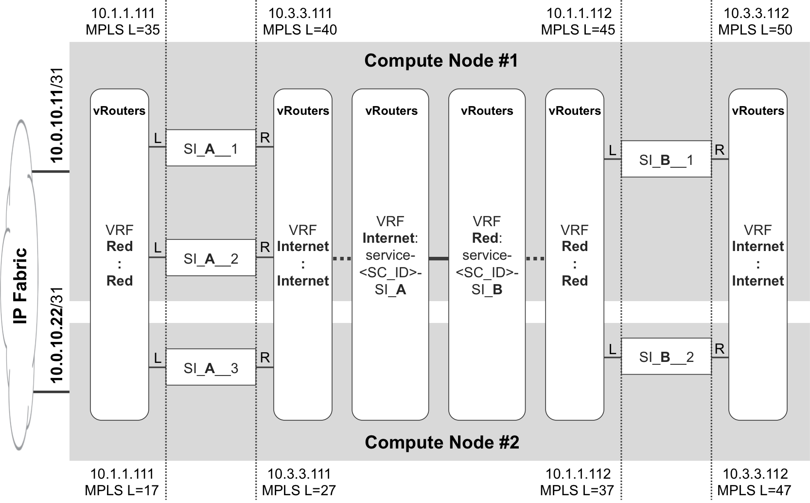
Figure 12-5. NFV scaling and redundancy
In OpenContrail configuration terms, you should check the scaling box on the Service Template configuration, and then define a new service instance with a number of instances greater than one. In this example, two service instances are defined:
-
SI_A, with a number of instances equal to three.
-
SI_B, with a number of instances equal to two.
The SI_A__# and SI_B__# VMs are dynamically created upon the previous configuration. From a functional point of view, this SFC is very similar to a simple SFC; it just has more than one VM per stage. The result is more horsepower and a higher level of resiliency. Here are some key observations from Figure 12-5:
-
VMs are distributed across compute nodes.
-
Shared IP addressing is supported. For example, all the left interfaces of SI_A instances have IP address 10.1.1.111. And they also get the same MAC address in this flavor of service instance.
-
MPLS labels are locally assigned by each vRouter, so they do not necessarily have the same value on different compute nodes. For example, if vRouter_1 receives an MPLS packet with label 45, it pops the label and sends the packet to the left interface of one of its SI_B instances. And there is only one such instance in compute node 1, namely SI_B__1. The outcome on vRouter_2 would be different, again due to the local significance of MPLS labels.
NFV Scaling and Redundancy—Load Balancing
OK, so MPLS labels are different across vRouters. On the other hand, vRouter_1 maps the same MPLS label (35) to the left interfaces of both SI_A__1 and SI_A__2. And it also maps MPLS label 40 to the right interfaces of the same VMs. The reason: these VMs belong to a common scaled service instance.
In Example 12-3, we can see these routes from the point of view of the gateway node.
Example 12-3. Route pointing to an SFC—Junos (DC-GW)
1     juniper@DC-GW> show route receive-protocol bgp 10.0.10.3
2                    table Red 0/0 exact
3
4     [...]
5     * 0.0.0.0/0 (1 entry, 1 announced)
6          Route Distinguisher: 10.0.10.11:15
7          VPN Label: 35
8          Nexthop: 10.0.10.11
9     [...]
10         Route Distinguisher: 10.0.10.22:15
11         VPN Label: 17
12         Nexthop: 10.0.10.22
The IP address of the control node is 10.0.10.3 (line 1), whereas the vRouter addresses are 10.0.10.11 (lines 6 and 8) and 10.0.10.22 (lines 10 and 12).
Because OpenContrail uses a <ROUTER_ID>:<VPN_ID> Route Distinguisher (RD) format, the gateway node considers the two IP VPN routes 10.0.0.11:15:0/0 and 10.0.0.22:15:0/0 as different. Thanks to that, the gateway node can load-balance the traffic across the two available next hops: vRouter_1 label 35 and vRouter_2 label 17.
Let’s look at how vRouter_1 effectively load-balances flows between the left interfaces of SI_A__1 and SI_A__2 (Example 12-4).
Example 12-4. Load balancing across service instances—OpenContrail (vRouter_1)
1     root@compute_node_1:~# mpls --get 35
2     MPLS Input Label Map
3        Label    NextHop
4     -------------------
5           35        58
6
7     root@compute_node_1:~# nh --get 58
8     Id:58  Type:Composite  Fmly: AF_INET
9     Flags:Valid, Policy, Ecmp, Rid:0  Ref_cnt:2 Vrf:3
10                  Sub NH(label): 41(22) 57(41)
11
12    root@compute_node_1:~# nh --get 41
13    Id:41  Type:Encap  Fmly: AF_INET  Flags:Valid, Rid:0 Ref_cnt:4 Vrf:3
14                  EncapFmly:0806 Oif:7 Len:14
15                  Data:02 8a 40 57 28 43 00 00 5e 00 01 00 08 00
16
17    root@compute_node_1:~# nh --get 57
18    Id:57  Type:Encap  Fmly: AF_INET  Flags:Valid, Rid:0 Ref_cnt:4 Vrf:3
19                  EncapFmly:0806 Oif:5 Len:14
20                  Data:02 8a 40 57 28 43 00 00 5e 00 01 00 08 00
This is a sample of the commands available on the vRouter command-line interface (CLI). These are plain commands that you can run on the host OS shell, and they are further documented on the OpenContrail website. But back to the example, incoming packets with MPLS label 35 are processed with an Equal-Cost Multipath (ECMP) next hop (line 9) containing two sub next hops. These have different outgoing interfaces (lines 14 and 19), as can be expected, because they point to two different VMs: SI_A__1 and SI_A__2. Conversely, they have the same encapsulation. Lines 15 and 20 can be decoded as shown here:
-
Destination MAC address 02:8a:40:57:28:43, shared by both VMs’ left interfaces
-
Source MAC address 00:00:5e:00:01:00, on the vRouter side
-
Ethertype 0x0800 (IPv4)
NFV—load-balancing assessment
Load balancing is great because it makes it possible to distribute different left-to-right packets across all of the six available paths. Indeed, a given left-to-right packet stream can traverse SI_A__X and SI_B__Y, where X has three possible values (1, 2, 3) and Y has two possible values (1, 2). In total, there are six possible combinations.
Likewise, right-to-left packets also have six possible paths. And here comes the challenge. Many network services—actually, the majority of them—require flow symmetry. If the upstream half-flow traverses SI_A__1 and SI_B__2, return packets must traverse SI_B__2 and SI_A__1. Otherwise, the flow is either disrupted or the appropriate services are not applied to it.
OpenContrail vRouters have flow awareness, and they can redirect packets appropriately. This topic is a complex one and OpenContrail website has interesting articles about it that you can read at http://www.opencontrail.org.
Service Instance Flavors
Until now, all of this chapter’s examples feature service instances cloned from a service template that, in OpenContrail technology, is of type [In-Network, Firewall].
The term Firewall refers here to a VM with left and right interface, as compared to a VM with just one service interface (Analyzer). The VM itself does not need to be a firewall—or to implement a firewall service—for that, at all.
In-Network Service Instances
The term In-Network is a much more interesting concept. In-Network means that the service instances (VMs) have IP capability on their left and right interfaces. In other words, they provide L2 termination and they process packets at L3. So VMs need some kind of L3 forwarding intelligence to avoid disrupting the chain’s forwarding plane. The following alternatives are available for In-Network service instances:
-
Make the VMs run in interface-based forwarding mode. A packet that enters the VM on one service interface (left, right) must exit—unless it is discarded by the VM—via the other (right, left) service interface. Of course, this imposes a requirement on the forwarding logic implemented by the VM. That being said, from a pure NFV perspective, it is the best practice.
-
Bring routing awareness to the VM. One option is to let OpenContrail include route prefixes in its DHCP offer, as described in RFC 3442 - The Classless Static Route Option for DHCP version 4. In this way, a service instance can learn how to reach certain destination networks through its left or right interface.
-
Letting the VM run dynamic routing protocols with other elements in the same tenant; although not a trivial operation, it is also an option.
Apart from In-Network, there are two other service instance types in OpenContrail.
In-Network-NAT Service Instances
This service instance flavor is similar to In-Network, with one big difference: the left VN prefixes are not leaked into the right VN. Back to the original example in Figure 12-2, the subscriber prefix 192.0.2.0/24 would not be leaked to the Internet VRF. This is perfectly fine if the service instance is performing a NAT function: there is no need to expose the inner (left) private address to the (right) public network domain.
To achieve end-to-end connectivity, the right VN must have the appropriate routes toward the public NAT pool. These routes must be installed at—and advertised by—the NVO. They should point to the NAT service instance’s right-facing interface. This is definitely possible in OpenContrail but beyond the scope of this MPLS book.
Transparent Service Instances
The best practice is L3. In that sense, it is preferred to run service VMs in the In-Network mode. But if a given service VM performs L2 bridging on transit packets, the service instance must be defined as transparent. One immediate implication is that MAC addresses are no longer shared.
When a service instance runs in transparent mode, the vRouter-VM link is VLAN-tagged allowing for the same service instance to be used in different SFCs, each with its own VLAN tag. Thus, the VM must be aware that traffic can arrive tagged with any VLAN tag and that tag must be preserved when switching frames between the left and the right interface. Back to Example 12-4, if the service instances were transparent you would see ethertype 0x8100 and additional bytes to encode the VLAN tags on lines 15 and 20.
Network Service Function Outside a VM or Container
VMs and containers in the NVO do not necessarily implement all the Network Service Functions (NSFs). Here are some other frequent alternatives:
-
Implementing the network function at the vRouter. The feature set of vRouters and vSwitches in different NVO solutions keeps growing. Sometimes, the NVO infrastructure can implement a service directly instead of relying on a VM for that.
-
Using an external device or appliance, which is called a Service Node in OpenContrail terminology. Very frequently, a data center may have physical network or security elements that need to be integrated in the SFC.
This book does not cover the integration of these two types of network service functions with VM-based SFCs like the one illustrated throughout this chapter.