
Chapter 14. TE Bandwidth Reservations
Bandwidth reservations are an essential tool that you can use to do the following:
-
Avoid link congestion in networks with high-volume traffic, such as ISP backbones.
-
Ensure that the most critical applications have their bandwidth resources available.
This chapter covers the control plane required to perform bandwidth reservations. To date, the only protocol that is capable of actually reserving bandwidth in a network is RSVP-TE. Most forwarding plane details—in particular, fine-grained mapping of certain traffic to certain LSPs—are specific to each platform and beyond the scope of this book.
Note
This book does not cover DiffServ-TE. It is not widely deployed.
The Traffic Engineering (TE) link constraints that are discussed in Chapter 13 are very simple, and are represented by single numbers. In this chapter, you will discover more complex TE use cases, with composite TE link attributes such as bandwidth.
TE Static Bandwidth Constraints
The next TE link characteristic is bandwidth. Bandwidth is a little bit special. It is no longer a single attribute, but a set of attributes that you can find in the IGP’s link-state databases, in the Traffic Engineering Database (TED) and in the RSVP-TE messages.
TE Bandwidth Attributes
Let’s have a look at the different attributes that comprise the TE bandwidth.
Maximum bandwidth (4 octets)
This is the physical interface bandwidth (e.g., 1.25 GByte/s for a 10GE interface). Typically, this parameter is inherited from the interface bandwidth, but you can also set it manually. This parameter is not used in TE calculations and is purely informational.
Maximum reservable bandwidth (4 octets)
This is the bandwidth that RSVP-TE is allowed to reserve. It can be bigger than the Maximum Bandwidth (if you allow RSVP-TE oversubscription), equal to the Maximum Bandwidth (if all the interface bandwidth can be taken by RSVP-TE) or smaller than the Maximum Bandwidth (if you don’t allow RSVP-TE to take the full interface bandwidth). Typically, this parameter is manually configured. If not explicitly configured, the default value in Junos is the full interface bandwidth, whereas in IOS XR, it is zero.
Unreserved bandwidth per priority level (8 x 4 octets)
This is the set of eight counters that keep track of the available bandwidth for each RSVP-TE priority (priority will be discussed later in this chapter). Although the previous two parameters are rather stable (after you start the IGP, the same values are advertised continuously), unreserved bandwidth changes dynamically. Each time a new LSP with bandwidth reservation is established, or existing LSPs with bandwidth reservation are torn down, or they change their bandwidth reservations, the value of this parameter is adjusted and flooded via the IGP. Actually, typical IGP implementations set some thresholds to suppress flooding when bandwidth changes are not significant.
Putting it all together, IGP distributes bandwidth information using 40 octets (4 + 4 + 32), plus normal TLV headers. All the bandwidth values are in bytes/s (not bits/s). Bandwidth was introduced with the initial TE extensions in OSPF and in IS-IS.
Default TE Interface Bandwidth
After this small bit of theory, let’s get into the lab. First, the default behavior of Junos and IOS XR is completely different. As mentioned previously, without any explicit RSVP-TE bandwidth configuration, Junos allows RSVP-TE to utilize the full interface bandwidth, whereas IOS XR does not allow RSVP-TE to reserve any bandwidth.
Example 14-1. RSVP interface status with default bandwidth on PE1 (Junos)
juniper@PE1> show rsvp interface
RSVP interface: 2 active
               Active Subscr- Static   Available Reserved Highwater
Interface   St resv   iption  BW       BW        BW       mark
ge-2/0/2.0  Up      8   100%  1000Mbps 1000Mbps  0bps     0bps
ge-2/0/3.0  Up      4   100%  1000Mbps 1000Mbps  0bps     0bps
Example 14-2. RSVP interface status with default bandwidth on PE2 (IOS XR)
RP/0/0/CPU0:PE2#show rsvp interface
(...)
Interface  MaxBW (bps)  MaxFlow (bps) Allocated (bps) MaxSub (bps)
---------- ------------ ------------- --------------- ------------
Gi0/0/0/2            0              0        0 (  0%)            0
Gi0/0/0/3            0              0        0 (  0%)            0
Basic RSVP-TE Bandwidth Reservation
Figure 14-1 shows three LSPs: PE1→PE3, PE2→PE4, and PE2→P5. Initially, only the two first LSPs are configured, and this time an explicit bandwidth reservation is included.
Let’s request 500 kbps for PE1→PE3 and 700 kbps for PE2→PE4, as shown in Figure 14-1 and presented in Example 14-3 and Example 14-4. Note that, in IOS XR, you specify bandwidth in kbps, whereas in Junos it’s bps.
Example 14-3. RSVP-TE bandwidth request on PE1 (Junos)
protocols {
    mpls label-switched-path PE1--->PE3 bandwidth 500k;
}
Example 14-4. RSVP-TE bandwidth request on PE2 (IOS XR)
interface tunnel-te44
 signalled-bandwidth 700
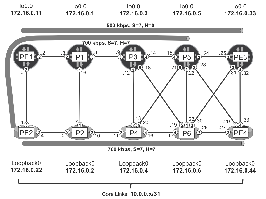
Figure 14-1. TE with bandwidth constraints
RSVP-TE tries to signal the tunnel, but now CSPF verifies if the additional constraint (bandwidth) is fulfilled. That is, the LSP is established only if all the links on the path have at least 500 (or 700) kbps free bandwidth. Free in this context means bandwidth that can be reserved by RSVP-TE, and for the moment, has nothing to do with the bandwidth utilized by actual traffic.
Example 14-5. RSVP-TE LSP status on PE1 and PE2
1     juniper@PE1> show mpls lsp name PE1--->PE3 detail | match <pattern>
2       From: 172.16.0.11, State: Up, ActiveRoute: 0, LSPname: PE1--->PE3
3         Bandwidth: 500kbps
4
5     RP/0/0/CPU0:PE2#show mpls traffic-eng tunnels 44 | include <pattern>
6         Admin:    up Oper: down   Path: not valid   Signalling: Down
7           Info: No path to destination, 172.16.0.44 (bw)
8         Bandwidth Requested: 700 kbps  CT0
The PE1→PE3 tunnel is up (line 2), whereas the PE2→PE4 tunnel is down (line 6). Apparently, between PE2 and PE4 there is no path for which at least 700 kbps are free (meaning reservable by RSVP-TE).
Explicit TE interface reservable bandwidth
So, as shown in Example 14-6 and Example 14-7, let’s configure consistent bandwidth reservations through the network and allow 10 Mbps for RSVP-TE on each link in the network. You can simply enhance existing GR-RSVP configuration groups to include the new bandwidth parameters.
Example 14-6. RSVP-TE link bandwidth configuration (Junos)
1     groups {
2         GR-RSVP {
3             protocols rsvp interface "<*[es]*>" subscription 1;
4     }}}
5     protocols rsvp apply-groups GR-RSVP;
Example 14-7. RSVP-TE link bandwidth configuration (IOS XR)
1     group GR-RSVP
2      rsvp
3       interface 'GigabitEthernet.*'
4        bandwidth 10000
5     !
6     rsvp apply-group GR-RSVP
7     !
In Junos, you can specify the percentage of interface bandwidth (line 3 in Example 14-6) that can be used for RSVP-TE reservations, or set explicit limits in bps—1% of 1 Gbps is 10 Mbps, so the result is the same. However, in IOS XR, you simply specify the limit in kbps (line 4 in Example 14-7).
With this configuration in place, the PE2→PE4 LSP is now up.
Example 14-8. Tunnel status on PE2 (IOS XR)
RP/0/0/CPU0:PE2#show mpls traffic-eng tunnels 44 | include <pattern>
    Admin:    up Oper:   up   Path:  valid   Signalling: connected
    Bandwidth Requested: 700 kbps  CT0
Because there are 10 Mbps available to reserve on every link by RSVP-TE, you can establish the tunnel with the 700 kbps requirement without any problems, and routers update the link bandwidth reservations accordingly.
Example 14-9. RSVP interface status with explicit bandwidth
juniper@PE1> show rsvp interface
RSVP interface: 2 active
               Active Subscr- Static   Available Reserved Highwater
Interface   ST resv   iption  BW       BW        BW       mark
ge-2/0/2.0  Up      8     1%  1000Mbps 9.5Mbps   500kbps  500kbps
ge-2/0/3.0  Up      3     1%  1000Mbps 10Mbps    0bps     0bps

RP/0/0/CPU0:PE2#show rsvp interface
(...)
Interface MaxBW (bps) MaxFlow (bps) Allocated (bps) MaxSub (bps)
--------- ----------- ------------- --------------- ------------
Gi0/0/0/2        10M            10M     700K (  7%)            0
Gi0/0/0/3        10M            10M       0  (  0%)            0
You can see that now the Maximum Reservable Bandwidth is 10 Mbps on each link (Junos: AvailableBW + ReservedBW; IOS XR: MaxBW). Also, you can see the currently reserved bandwidth on each interface (Junos: ReservedBW; IOS XR: Allocated). This information is distributed via the IGP, as demonstrated in Example 14-10.
Example 14-10. TE bandwidth announcements in IS-IS
1     juniper@PE1> show isis database PE1 extensive
2     (...)
3         IS extended neighbor: P1.00, Metric: default 1000
4           IP address: 10.0.0.2
5           Neighbor's IP address: 10.0.0.3
6           Local interface index: 337, Remote interface index: 335
7           Current reservable bandwidth:
8             Priority 0 : 9.5Mbps
9             Priority 1 : 9.5Mbps
10            Priority 2 : 9.5Mbps
11            Priority 3 : 9.5Mbps
12            Priority 4 : 9.5Mbps
13            Priority 5 : 9.5Mbps
14            Priority 6 : 9.5Mbps
15            Priority 7 : 9.5Mbps
16          Maximum reservable bandwidth: 10Mbps
17          Maximum bandwidth: 1000Mbps
18          Administrative groups:  0 <none>
19
20    RP/0/0/CPU0:PE2#show isis database PE2 verbose
21    (...)
22      Metric: 1000       IS-Extended P2.00
23        Affinity: 0x00000000
24        Interface IP Address: 10.0.0.4
25        Neighbor IP Address: 10.0.0.5
26        Physical BW: 1000000 kbits/sec
27        Reservable Global pool BW: 10000 kbits/sec
28        Global Pool BW Unreserved:
29          [0]: 10000    kbits/sec          [1]: 10000    kbits/sec
30          [2]: 10000    kbits/sec          [3]: 10000    kbits/sec
31          [4]: 10000    kbits/sec          [5]: 10000    kbits/sec
32          [6]: 10000    kbits/sec          [7]: 9300     kbits/sec
33    (...)
Both PE1 and PE2 advertise 10 Mbps as the links’ maximum reservable bandwidth (lines 16 and 27). Conversely, there are some differences when you look for the bandwidth available at each priority level. For the PE1→P1 link, the announced bandwidth for each priority is 9.5 Mbps (lines 8 through 15), whereas for the PE2→P2 link it is 10 Mbps for priority 0–6 (lines 29 through 32), and 9.3 Mbps for priority 7 only (line 32). This is yet another difference in the default implementation of Junos and IOS XR; let’s see its meaning after introducing some new concepts.
LSP Priorities and Preemption
If you now configure PE2→P5 (the remaining LSP from Figure 14-1) with a 700 kbps reservation, it has several available paths to choose. Let’s suppose that it uses the PE2→PE1 link and that completes all the LSPs shown in Figure 14-1.
Now, suppose that you configure yet another new PE2→P6 tunnel (not shown in Figure 14-1) with 9400 kbps bandwidth reservation. As you can see by looking at the bandwidth reservations on Figure 14-1, the new LSP’s setup would fail because there is no path with 9400 kbps of available bandwidth on all links. Specifically, all links adjacent to PE2 have available bandwidth less than 9400 kbps.
You can fix the problem by moving one of the small bandwidth LSPs to another link. For example, if you move the PE2→P5 LSP from the PE2→PE1 to the PE2→P2 link, the PE2→PE1 link would have 10 Mbps free bandwidth. This is enough for the new LSP requiring 9.4 Mbps to fit, at least on this link.
How can you achieve this? Well, one option is to manually reroute the PE2→P5 LSP, by setting an explicit path. However, in large networks with many LSPs in place, setting explicit paths everywhere can be a challenging task.
Therefore, let’s consider another approach: LSP preemption. With LSP preemption, you can designate some LSPs as more important, and other LSPs as less important. More-important LSPs can preempt (kick-out or remove: choose your verb) existing less-important LSPs. Let’s suppose that you designate the high-bandwidth PE2→P6 LSP to be more important that the PE2→P5 LSP. In this case, the PE2→P6 LSP preempts the PE2→P5 LSP. As a result of this preemption, the PE2→P5 LSP is removed from the PE2→PE1 link. When the PE2→P5 LSP is calculated again, PE2 signals it over a different path. As you can see in Figure 14-2, in the end every configured LSP successfully comes up.
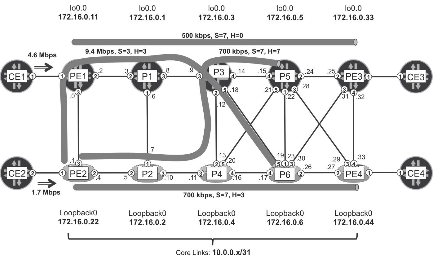
Figure 14-2. TE with bandwidth constraints and preemption
Setup and Hold priorities
Now, how can you configure the importance of an LSP? In TE, there is a concept of Setup and Hold priority. Numerically lower priority is better. Thus, when a new LSP is being signaled, in case of resource conflict (e.g., not enough bandwidth on a certain link) the Setup priority of the new LSP is compared to the Hold priority of the existing LSP. If it is numerically lower, the new LSP can preempt the existing LSP.
As shown next, the default settings for Setup and Hold priority are different in Junos and IOS XR.
Example 14-11. Default Setup and Hold priorities
juniper@PE1> show mpls lsp name PE1--->PE3 detail | match Priorities
    Priorities: 7 0

RP/0/0/CPU0:PE2#show mpls traffic-eng tunnels 44 | include Priority
    Bandwidth:      700 kbps (CT0) Priority:  7  7
What is the difference? In Junos, it is 7 (Setup) and 0 (Hold), whereas in IOS XR it is 7 for both Setup and Hold. It means that the LSPs signaled by Junos are by default rock-solid: after they are established, no other LSP can preempt them. Why? The Hold priority of Junos-signaled LSPs is 0, so it is not possible for another LSP to have a numerically lower Setup priority. IOS XR is just the opposite: the Hold priority is 7, so any LSP with Setup priority 0 through 6 can preempt such an LSP.
If you go back to Example 14-10, you will now understand why Junos and IOS XR advertised different free bandwidths. IOS XR advertised the full bandwidth (10 Mbps) available at priority level 0 through 6, meaning that any LSP with a Setup priority level 0 through 6 can take full bandwidth on the advertised link.
With that behind us, let’s configure a better (numerically lower) hold priority for PE2→PE4 LSP. This will make it more resistant to preemption by other LSPs.
Example 14-12. PE2→PE4 LSP priority configuration on PE2 (IOS XR)
interface tunnel-te44
 priority 7 3
With this configuration, the lines 29 through 32 from Example 14-10 would change to the following:
-
Priorities [0] to [2]: reservable bandwidth 10000 kbps
-
Priorities [3] to [7]: reservable bandwidth 9300 kbps
Now, let’s configure the PE2→PE6 tunnel, which is requesting 9.4 Mbps bandwidth, with Setup priority 3, as demonstrated in Figure 14-2 and in Example 14-13.
Example 14-13. PE2→P6 LSP priority configuration on PE2 (IOS XR)
interface tunnel-te6
 priority 3 3
To maintain LSP stability, the Hold priority cannot be worse (numerically higher) than the Setup priority. This is enforced by a commit check, on both IOS XR and Junos platforms. Therefore, 3 was configured for both Setup and Hold priorities.
Results of LSP preemption and resignaling
With its new Setup priority, the PE2→PE6 LSP will be able to preempt the PE2→P5 tunnel (Hold priority 7), but not the PE2→PE4 tunnel (Hold priority 3). Let’s check that.
Example 14-14. RSVP interface status after preemption on PE2 (IOS XR)
1     RP/0/0/CPU0:PE2#show rsvp interface
2     (...)
3     Interface   MaxBW (bps)  MaxFlow (bps) Allocated (bps) MaxSub (bps)
4     ----------- ------------ ------------- --------------- ------------
5     Gi0/0/0/2           10M            10M    1400K ( 14%)            0
6     Gi0/0/0/3           10M            10M    9400K ( 94%)            0
The RSVP bandwidth reservations reported on the interfaces confirm that now all four of the LSPs in question, three of them initiated at PE2, are established. You can see the global LSP placement in Figure 14-2.
In Junos, you also can configure RSVP-TE LSP priorities by using the priority <SETUP> <HOLD> keyword, this time under the mpls label-switched-path <NAME> stanza. The logic is similar to IOS XR, we’ll skip it for brevity.
Note
You can achieve an enhanced LSP distribution logic with the help of a central controller. See Chapter 15 for more details.
Traffic Metering and Policing
Now, let’s push some traffic through the PE1→PE3 and PE2→PE4 LSPs. Suppose that the actual utilization of both PE1’s and PE2’s uplinks exceed the reserved LSP bandwidth (500 and 700 kbps, respectively). If you want to know what LSPs are contributing to the overall traffic rate, there are at least two handy operational commands that you can use:
-
For Junos:
show mpls lsp statistics -
For IOS XR:
show mpls forwarding
Although these commands are great, they do not really integrate with the TE logic of PE1 and PE2. If you really want to make TE traffic-aware, you need at the very least to add some configuration to collect traffic statistics on a per-LSP basis.
Example 14-15. LSP bandwidth monitoring on PE1 (Junos)
1     protocols mpls {
2         statistics {
3             file mpls.stat size 100m files 10;
4             interval 120;
5             auto-bandwidth;
6         }
7         label-switched-path PE1--->PE3 {
8             auto-bandwidth monitor-bandwidth;
9     }}
Example 14-16. LSP bandwidth monitoring on PE2 (IOS XR)
1     interface tunnel-te44
2      auto-bw
3       collect-bw-only
4     !
5     mpls traffic-eng
6      auto-bw collect frequency 2
This configuration enables the collection of average bandwidth samples every 120 seconds (Example 14-15), or in other words, every 2 minutes (Example 14-16). As a result, the TE logic is aware of the bandwidth that is actually used by the LSP.
Example 14-17. LSP bandwidth utilization
juniper@PE1> show mpls lsp name PE1--->PE3 detail | match <pattern>
  Max AvgBW util: 4.65488Mbps
..
RP/0/0/CPU0:PE2#show mpls traffic-eng tunnels 44 | include <pattern>
      Highest BW: 1738 kbps   Underflow BW: 0 kbps
Your LSPs are consuming much more bandwidth than the requested 500 (or 700) kbps! This simple example shows that there is no admission control for traffic entering TE tunnels. TE bandwidth is simply an accounting term, but it is not coupled with any policing by default. It is like requesting 700 tickets for a football game, and subsequently sending 1,738 people, hoping that there aren’t any ticket checks at the entrance to the stadium. And, in the case of RSVP-TE, there aren’t!
Therefore you need to take additional measures, and you basically have two options to ensure that the traffic demand and bandwidth accounting (TE bandwidth reservations) are aligned:
-
Limit the traffic entering TE tunnels (comparable to using football game ticket checks) to match the requested bandwidth.
-
Adjust TE tunnels bandwidth reservations to match the traffic demand (comparable to allocating more tickets for the football game).
This chapter will soon dive deep into the second model. Regarding the first model, as of this writing, it is implemented by Junos but not by IOS XR. Here is the Junos syntax:
Example 14-18. Automatic LSP policing configuration on PE1 (Junos)
protocols {
    mpls auto-policing class all drop;
}
This feature assigns policers to LSPs that automatically match each of the LSPs’ reserved bandwidth.
TE Auto-Bandwidth
So far in this chapter, all of the examples have relied on static bandwidth constraints. However, traffic patterns and bandwidth utilization are extremely dynamic. The rest of this chapter looks at ways to adapt the LSP layout based on the actual traffic.
Introduction to Auto-Bandwidth
As already mentioned, it is possible to adapt bandwidth reservations to the actual traffic demand. This is obviously gentler to traffic than admission control.
Doing it manually is not an option for large networks with thousands of LSPs, oscillating traffic patterns, and changing service demands. Therefore, it’s better to use automation for implementing adjustments. Two building blocks are required:
-
Traffic rate measurements per LSP (already described).
-
Periodic adjustments of RSVP-TE bandwidth reservations based on the measured traffic rates. This feature is called auto-bandwidth.
If a bandwidth adjustment is needed, the ingress PE takes into account the new bandwidth and runs CSPF again. If CSPF succeeds, the ingress PE resignals the LSP according to new path computation.
Note
Auto-bandwidth is an asynchronous process. Ingress Label Edge Routers (LERs) are distributed across the network and typically perform their own calculations and bandwidth adjustments, at their own timing.
If LER-1 performs a bandwidth adjustment, it can influence the next adjustment performed by LER-2. There is even a risk of “collision” when the two LERs try to simultaneously reserve resources on the same link. Although real experience in large providers shows that auto-bandwidth is robust and converges fine, it is also an opportunity for a central controller to bring synchrony to this process.
Both Junos and IOS XR support auto-bandwidth, but as usual, the terminology and the implementation details are different. The following subsections list the most important auto-bandwidth parameters for both vendors. Take the time to carefully read this short “user guide” because these concepts are mandatory to understand the practical example.
Collection (sampling) interval
- Junos
set protocols mpls statistics interval <seconds>- IOS XR
mpls traffic-eng auto-bw collect frequency <minutes>
This timer controls how often the router collects traffic rates for every LSP that has the auto-bandwidth feature turned on. These measurements, called bandwidth samples, are traffic averages calculated for the collection interval. They are stored in an internal database for MPLS statistics (in Junos, it is a logfile whose properties you can tune).
Application (adjustment) interval
- Junos
set protocols mpls label-switched-path <name> auto-bandwidth adjust-interval <seconds>- IOS XR
interface tunnel-te<id> auto-bw application <minutes>
Typically, the adjustment interval is a multiple of the sampling interval; so several samples are collected for the LSP within each adjustment interval. When the adjustment timer expires, there is an adjustment event. The router looks at all of the samples that have been collected within the last adjustment interval and chooses the one with a maximum value: the maximum bandwidth sample. This value is compared to the currently signaled LSP bandwidth and this comparison may cause the RSVP-TE LSP to be resignaled in order to update the reserved bandwidth. Whether this update takes place depends on whether the bandwidth has changed enough (see the following parameter).
Application (adjustment) threshold
- Junos
set protocols mpls label-switched-path <name> auto-bandwidth adjust-threshold <percent>- IOS XR
interface tunnel-te<id> auto-bw adjustment-threshold <percent> min <kbps>
This is defined as a percentage of the current tunnel’s reserved bandwidth. In IOS XR, optionally, you also can specify an absolute bandwidth difference.
At the end of each adjustment interval, the router compares the following two values:
-
The currently reserved LSP bandwidth
-
The maximum bandwidth sample from the expired adjustment interval
If the difference is larger than the configured thresholds, the LSP is resignaled with a new bandwidth value that equals the maximum bandwidth sample.
Note
It is assumed that you understand the connection between application and adjustment, and collection and sampling, from this point on.
Overflow detection
- Junos
set protocols mpls label-switched-path <name> auto-bandwidth adjust-threshold-overflow-limit <number>- IOS XR
interface tunnel-te<id> auto-bw overflow threshold <percent> min <kpbs> limit <number>
If the rate of the traffic entering an LSP drastically increases, the LSP bandwidth should be resized quickly, without having to wait for the expiry of an adjustment interval.
At the end of each sampling interval, the router compares the following two values:
-
The currently reserved LSP bandwidth.
-
The average bandwidth sample from the expired sampling interval.
If the difference is larger than the configured thresholds, the current sample is considered an overflow sample. After a configurable number of consecutive overflow samples, the adjustment interval prematurely ends. An adjustment event takes place and the router resignals the LSP with a new bandwidth value that equals the maximum bandwidth sample. This configurable number of consecutive overflow samples is called an overflow limit.
For overflow detection, Junos reuses the threshold parameter (percentage) specified for adjustment thresholds, whereas with IOS XR, you can specify separate parameters.
Underflow detection
- Junos
set protocols mpls label-switched-path <name> auto-bandwidth adjust-threshold-underflow-limit <number>- IOS XR
interface tunnel-te<id> auto-bw underflow threshold <percent> min <kpbs> limit <number>
This is similar to overflow detection, but it works in the opposite direction. When the traffic rate entering the tunnel significantly lowers within the current adjustment interval, the tunnel bandwidth can be decreased automatically without waiting for the current adjustment interval to expire.
Requested bandwidth minimum and maximum limits
- Junos
set protocols mpls label-switched-path <name> auto-bandwidth minimum-bandwidth <bps> maximum-bandwidth <bps>- IOS XR
interface tunnel-te<id> auto-bw bw-limit min <kbps> max <kbps>
The auto-bandwidth feature can dynamically change LSP bandwidth reservations within certain limits. These commands set the limits.
Auto-Bandwidth in Action
The meaning of all these auto-bandwidth parameters might be difficult to understand at first glance, so let’s discuss the example presented in Figure 14-3.
Let’s assume the following parameters:
-
Collection (sampling) interval: 2 minutes (120 seconds)
-
Application (adjustment) interval: 20 minutes (1200 seconds) → 10 times the collection (sampling) interval
-
Requested minimum and maximum bandwidth: 1 kbps and 10 Mbps
-
Adjustment threshold: 10%, minimum 0.1 Mbps
-
Overflow threshold: 10%, minimum 0.1 Mbps
-
Overflow limit: 3
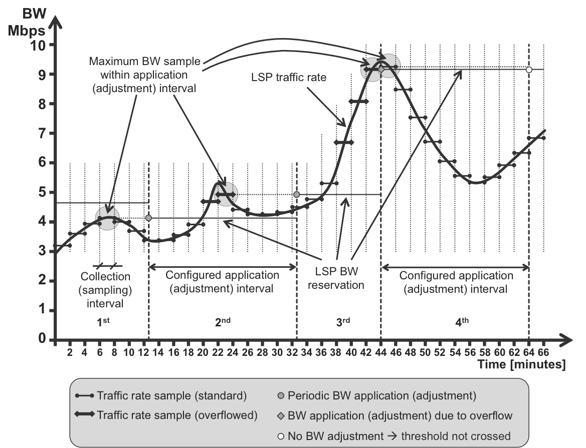
Figure 14-3. Auto-bandwidth in action
Warning
These timers are set quite aggressively for testing purposes, but they are not suitable for a scaled production environment.
Also, let’s assume that the tunnel has already been established for some time, so there are some traffic rate samples collected before (not shown in the Figure 14-3). There is some (around 4.7 Mbps) existing bandwidth reservation already in place.
Figure 14-3 begins with the six last traffic rate samples from the first application interval. Each sample is collected every 2 minutes, so here you see the last 12 minutes (out of 20) from this application interval. Each collected sample is an average rate of traffic entering the monitored LSP. The average is calculated over the sampling interval (2 minutes).
Now, the sample at T=8 is the highest, with around 4.0 Mbps (let’s assume that the not-visible four samples from the first adjustment interval are below 4.0 Mbps, too). The first application interval expires slightly after T=12. The bandwidth difference between the current bandwidth reservation (around 4.7 Mbps) and the maximum bandwidth sample (around 4.0 Mbps) is higher than the configured adjustment threshold (10% and 0.1 Mbps). Further, 4.7 Mbps is within the configured minimum and maximum (1 and 10 Mbps) limits. Therefore the router resignals the LSP, requesting around 4.0 Mbps bandwidth reservation only.
In the second application interval, the 10 bandwidth samples are collected again. Note that samples at T=22 (BW≈4.7) and T=24 (BW≈5.0) are above these two values:
-
4.1 x 110% = 4.4, the current bandwidth reservation adjusted to the 10% threshold.
-
4.0 + 0.1 = the current bandwidth reservation plus the minimum overflow difference.
These two samples are therefore considered as overflow samples.
However, the next sample (BW≈4.3), at T=26, is back below the overflow threshold. Therefore it is a standard sample. Because the configured overflow limit requires three consecutive overflow samples, the overflow-based bandwidth adjustment is not triggered. The bandwidth is adjusted based on the highest sample (T=24, BW≈5.0) only after T=32, when the configured application interval ends.
In the third application interval, the sample at T=38 is higher (BW≈5.3) than the current bandwidth reservation (BW≈5.0). However, it doesn’t cross the 10% overflow threshold; thus, it is not high enough to be considered as an overflow sample. The next three samples (T=40, T=42, and T=44), however, are well above the overflow threshold. Because three consecutive overflow samples are collected, the router doesn’t wait for the application timer to expire (after T=52). Instead, it prematurely expires the timer, resignals the bandwidth (based on the highest sample: T=44, BW≈9.0) reservation, and starts the new application interval immediately. Therefore, the rapid increase in bandwidth demand can be quickly addressed with bandwidth reservation resignaling, without the need to wait for the application interval to finish. Note, in this case, that if the bandwidth sample at T=44 were more than 10 Mbps, only 10 Mbps would be resignaled, due to the configured maximum bandwidth limit of 10 Mbps.
In the fourth application interval, only the first sample (T=46) is (slightly) higher than the current bandwidth reservation. All other samples are lower. However, because the difference between the first (maximum) sample and the current bandwidth reservation is small (less than the configured adjustment interval, which is 10%), when the application interval ends, the bandwidth is not resignaled. This helps to keep the RSVP-TE signaling load low, as the unimportant bandwidth changes don’t trigger the signaling.
It is worth noting that in the fourth application period you can see rapid bandwidth decreases of traffic flowing through the monitored LSP. However, this doesn’t trigger any bandwidth resignaling, because the underflow detection (similar to overflow detection) is not configured. If underflow detection had been configured with similar parameters to those used for overflow, the bandwidth would have been resignaled after T=54, following three consecutive underflow samples (T=50, T=52, T=54).
Auto-Bandwidth Configuration
That’s enough for the extended theory—let’s get into the lab now to configure automatic bandwidth adjustments in the network for all LSPs. Example 14-19 and Example 14-20 assume that the entire configuration discussed in this chapter (bandwidth reservations, LSP statistics, and LSP policing) is already removed before proceeding.
Example 14-19. Auto-bandwidth configuration on PE1 (Junos)
1     groups GR-LSP {
2         protocols mpls label-switched-path <*> {
3             auto-bandwidth {
4                 adjust-interval 1200;
5                 adjust-threshold 10;
6                 minimum-bandwidth 1k;
7                 maximum-bandwidth 10m;
8                 adjust-threshold-overflow-limit 3;
9                 resignal-minimum-bandwidth;
10    }}}
11    protocols mpls {
12        apply-groups GR-LSP;
13        statistics {
14            file mpls.stat size 100m files 10;
15            interval 120;
16            auto-bandwidth;
17    }}
Example 14-20. Auto-bandwidth configuration on PE2 (IOS XR)
1     group GR-LSP
2      interface 'tunnel-te.*'
3       auto-bw
4        bw-limit min 1 max 10000
5        overflow threshold 10 min 100 limit 3
6        adjustment-threshold 10 min 100
7        application 20
8     end-group
9     !
10    apply-group GR-LSP
11    !
12    mpls traffic-eng
13     auto-bw collect frequency 2
You can check that this configuration matches the parameters listed before Figure 14-3.
This book’s tests successfully achieved Junos and IOS XR interoperable auto-bandwidth.
Auto-Bandwidth Deployment Considerations
Both Junos and IOS XR use similar algorithms for automatic, periodic adjustments in bandwidth reservations. In the case of significant changes in detected traffic volume, both support very similar overflow and underflow detection mechanisms, to prematurely adjust reserved bandwidth without the need to wait for the application interval to end.
But in what scenarios is auto-bandwidth deployed? In many cases, auto-bandwidth is deployed in combination with preemption. You mark some LSPs (e.g., carrying voice or IPTV traffic) as important (numerically lower-priority values) and some other LSPs (e.g., carrying best-effort Internet traffic) as less important (numerically higher-priority values). For each LSP, you measure and periodically adjust the bandwidth reservation by using auto-bandwidth.
Now, CSPF tries to establish each LSP based on the TE metrics (shortest path to the destination), but it takes into account the bandwidth constraints enforced by auto-bandwidth. If there is enough unreserved bandwidth available on all the links on the shortest path, all of the LSPs will follow the shortest path. If there is not enough unreserved bandwidth, some LSPs will be placed over longer paths to the destination, where bandwidth is available. Which ones? Less-important LSPs. This all happens dynamically, without the need for user intervention. If bandwidth for some of the important LSPs increases, these LSPs will be able to kick-out (thanks to the configured priority levels) less-important LSPs from the shortest path. Less-important LSPs will be rerouted elsewhere in the network. And the reverse is also true. When the bandwidth used by important LSPs decreases, less-important LSPs might be placed back on the shortest path.
Another application of auto-bandwidth is load-balancing over equal or unequal-cost multipaths. For example, suppose that you might have multiple (not necessarily equal cost) paths available between PE-X and PE-Y, each path with a capacity of 10G, and you want to transport 15G worth of traffic between PE-X and PE-Y. You cannot transport it by using a single LSP, but you can create multiple LSPs and the ingress PE (PE-X) can perform load-balancing of traffic between the multiple LSPs. The auto-bandwidth feature will ensure that these multiple LSPs will be spread across multiple available paths if the bandwidth on a single path is not sufficient.
You can do load balancing, combined with auto-bandwidth, manually, so you define how many LSPs should be established between PE-X and PE-Y in the configuration. However, in large networks, with dynamically changing traffic patterns, this would be difficult from both a design and operation perspective. Therefore, Junos offers the next level of automation here; you not only measure and adjust LSP bandwidth reservations automatically, but you also increase or decrease the number of LSPs between two endpoints automatically. Let’s move on to this feature, which is called Dynamic Ingress LSP Splitting/Merging, which we’ll see in the next section.
Dynamic Ingress LSP Splitting/Merging
Dynamic Ingress LSP Splitting/Merging is based on RSVP-TE extensions defined in draft-kompella-mpls-rsvp-ecmp: Multi-path Label Switched Paths Signaled Using RSVP-TE. This draft introduces the new RSVP Association Object, which allows associating multiple child LSPs, called member LSPs, with a single parent LSP, called a container LSP. These are all Point-to-Point (P2P) LSPs: there is load balancing and not replication.
Figure 14-4 illustrates this concept. It is similar to Ethernet Link Aggregation Groups (LAG, IEEE 802.3ad), for which multiple physical Ethernet links are bundled together to make a single, aggregated Ethernet interface, consisting of multiple Ethernet link members. Now, members are LSPs, and the bundle is a container LSP.
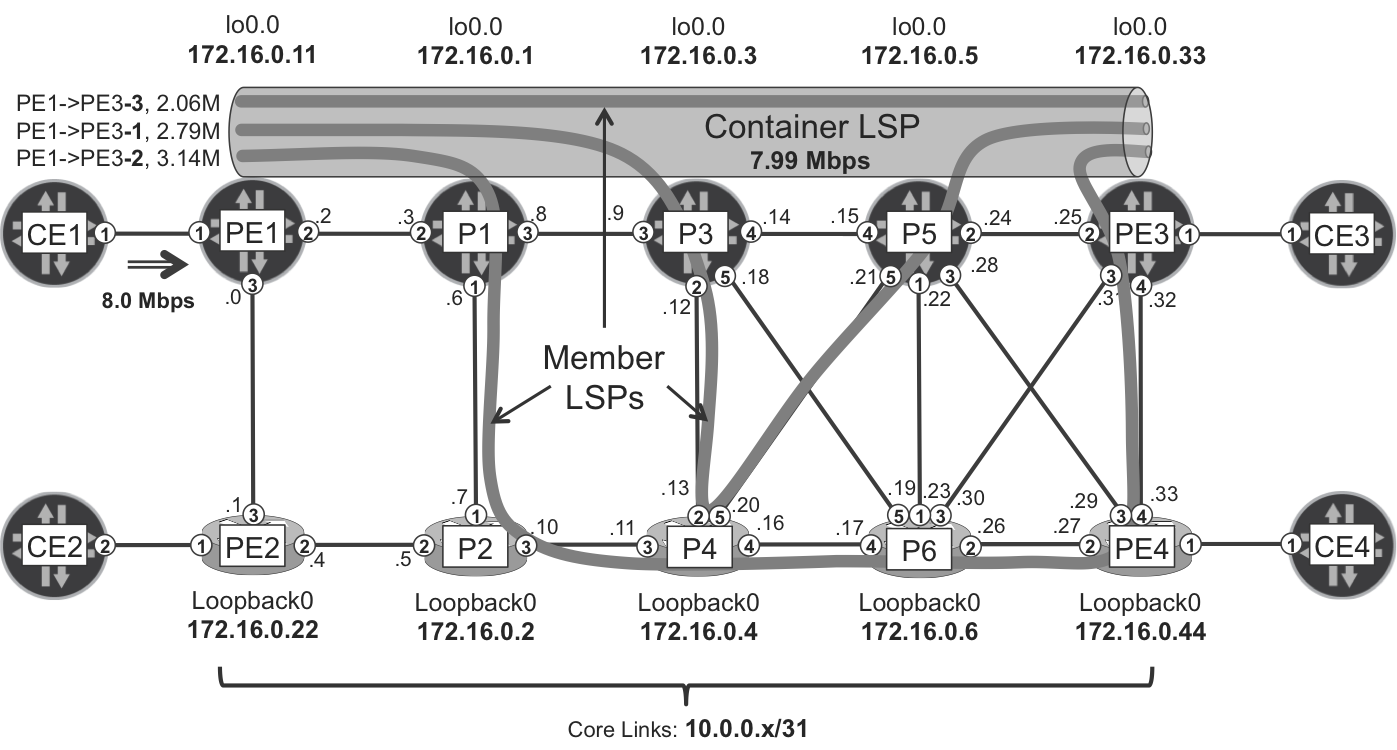
Figure 14-4. RSVP-TE multipath
As in Ethernet LAG, the ingress PE can load-balance the traffic across multiple member LSPs. Also like in Ethernet LAG, traffic is not always perfectly distributed between the members: this is an inherent limitation of hashing and load balancing.
You can place member LSPs over different paths across the network, so the traffic load between two endpoints (PE1 and PE3, in the example) can be spread across different links in the network. In the example topology presented in Figure 14-4, only the PE1→P1 link carries all three member LSPs. Some of the links carry two member LSPs, whereas most of the links carry only single member LSPs. The distribution of member LSPs is automatic, and greatly depends on the requested bandwidth of each LSP, and the bandwidth available for RSVP reservations on each link.
Dynamic Ingress LSP Splitting/Merging—Configuration
That’s the theory. Now let’s again get into the lab and remove the current PE1→PE3 LSP configuration from PE1, and then configure PE1 to use a container LSP, instead (see Example 14-21).
Example 14-21. PE1→PE3 container LSP configuration (Junos)
1     protocols mpls {
2         label-switched-path LSP-TEMPLATE {
3             template;
4             least-fill;
5             adaptive;
6             auto-bandwidth {
7                 adjust-interval 600;
8                 adjust-threshold 10;
9                 minimum-bandwidth 1k;
10                maximum-bandwidth 10m;
11                adjust-threshold-overflow-limit 3;
12                resignal-minimum-bandwidth;
13            }
14        }
15        container-label-switched-path PE1--->PE3 {
16            label-switched-path-template LSP-TEMPLATE;
17            to 172.16.0.33;
18            splitting-merging {
19                maximum-member-lsps 4;
20                minimum-member-lsps 1;
21                splitting-bandwidth 4m;
22                merging-bandwidth 2m;
23                normalization normalize-interval 1200;
24    }}}
Notice that instead of label-switched-path PE1--->PE3, you now have container-label-switched-path PE1--->PE3 (line 15). Likewise, the operational commands begin with show mpls container-lsp.
You can create templates for container LSPs (lines 2 through 14) describing common LSP characteristics, including auto-bandwidth parameters or other TE constraints. LSP-TEMPLATE is not a standard LSP definition: it includes the keyword template (line 3) instead of the keyword to. The template can be used later under the container LSP configuration stanza (line 16) so that the dynamically created member LSPs can inherit the parameters from the template.
Dynamic Ingress LSP Splitting/Merging in Action
Figure 14-4 shows a real lab test performed during this book’s writing. The traffic generator was sending an average of 8.0 Mbps, but this value was fluctuating a bit. At the time the picture was taken, the container LSP PE1→PE3 was transporting a total 7.99 Mbps of traffic, distributed across its member LSPs. Each of these member LSPs actually transported a different traffic rate due to the intrinsic imperfection of load balancing. So if the instantaneous bandwidth was 7.99 Mbps, why are there three member LSPs? Let’s answer this question fully.
Example 14-21 contains a completely new configuration stanza that controls the LSP splitting/merging behavior (lines 18 through 23):
-
Minimum (1) and maximum (4) number of member LSPs within a container LSP (lines 19 and 20)
-
Minimum (
merging-bandwidth 2m) and maximum (splitting-bandwidth 4m) bandwidth of a single member LSP (lines 21 and 22) enforced during each normalization event -
Normalization interval duration in seconds (line 23): 1200 seconds or 20 minutes.
At the end of each normalization interval, the system decides if the existing member LSPs should be merged or split. Figure 14-5 provides a correlation between the various intervals (auto-bandwidth sampling interval, auto-bandwidth adjustment interval, and LSP splitting/merging normalization interval) used in this dynamic process.
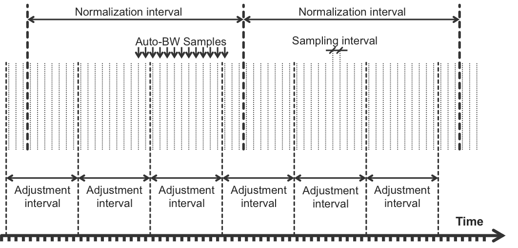
Figure 14-5. Interval correlations in dynamic LSP splitting/merging
Given the parameters from Example 14-21, and with a current aggregate bandwidth of 7.99 Mbps, there are two options:
-
3 (member LSPs) x 2.66 Mbps (each member LSP) approximately
-
2 (member LSPs) x 3.99 Mbps (each member LSP) approximately
Both options are valid (the number of member LSPs is between 1 and 4, and the member LSP’s bandwidth is between 2 and 4 Mbps). Here, the second option would normally be preferred because it requires the lowest number of member LSPs. However, there are three member LSPs. Why? Because the traffic generator was sending 8 Mbps on average, and one of the bandwidth samples collected during the last adjustment interval resulted in an aggregate of 8.01 Mbps.
Dynamic bandwidth calculations for splitting/merging are made according to the maximum bandwidth samples collected during the last normalization interval. With the parameters in Example 14-21, the only way to distribute 8.01 Mbps is to have three member LSPs.
Now imagine that the traffic generator brings down the traffic rate from 8 Mbps to 7.5 Mbps. After the next normalization interval (2 minutes) fully expires, the maximum bandwidth sample is around 7.5 Mbps and there are two options to distribute this traffic:
-
3 (member LSPs) x 2.50 Mbps (each member LSP)
-
2 (member LSPs) x 3.75 Mbps (each member LSP)
Both options are valid, but the second option will be used because this is the option with the lowest number of member LSPs. At this point, the container LSP brings one member LSP down and resignals the two other member LSPs with 3.75 Mbps.
Now imagine that the average bandwidth goes up to 15 Mbps. In this case, one simple LSP would never be able to reserve all the bandwidth because the links’ maximum reservable bandwidth is 10 Mbps. Only a container LSP with four member LSPs would satisfy the requirements. This is a key benefit of the new model.
Dynamic Ingress LSP Splitting/Merging and Auto-Bandwidth
Normalization (splitting or merging) starts assuming perfect load balancing; thus, the bandwidth initially requested during the normalization event is equal on all member LSPs. Then, standard auto-bandwidth mechanisms can further adjust the bandwidth reservation on each member LSP, based on the traffic statistics collected separately for each member LSP. As already discussed in “TE Auto-Bandwidth” this automatic adjustment can be:
-
A periodic bandwidth adjustment, which is separately tracked for each member LSP.
-
An ad hoc bandwidth adjustment, if traffic volume inside the member LSP significantly changes and overflow/underflow detection is enabled.
As of this writing, overflow/underflow detection mechanisms for the LSP splitting/merging feature were not implemented in Junos. Therefore, LSP normalization (splitting or merging) occurred only at scheduled intervals, without the possibility for faster reaction in case of significant changes in traffic volumes. However, you can definitely adjust member LSPs’ bandwidth upon an overflow/underflow condition.