
Chapter 3. Layer 3 Unicast MPLS Services
So far, this book has illustrated the primary role of MPLS: building tunnels (LSPs) across the service provider (SP) or the data center core in order to transport packets. In previous examples, the ingress PE performs a route lookup on each IPv4 packet before placing it on an LSP. This route lookup process takes into account Layer 3 (L3) fields contained in the IPv4 header; and the user packets are unicast—destined to a single host. Putting it all together, IPv4 Internet Transit over MPLS is an L3 Unicast MPLS Service. It is, historically speaking, the first MPLS service and in terms of volume it also remains the most widely used.
IPv4 Internet over MPLS is an unlabeled service, in the sense that packets typically have no MPLS label when they arrive to the egress (service) PE. While in the LSP, packets only carry transport labels, but no service labels. What is a service label? It is simply an MPLS label that identifies a service. At first glance, it is impossible to distinguish transport labels from service labels: they look the same. The difference lies in the way Label Switch Routers (LSRs) and Label Edge Routers (LERs) interpret them, as determined by the signaling process: when an LSR/LER advertises a label, it is also mapping it to something with a precise meaning.
If an MPLS service is labeled, the ingress PE typically pushes a stack of two MPLS headers—as long as the egress PE is more than one hop away. The outer and the inner headers contain a transport and a service label, respectively. Later in the path, the penultimate LSR pops the transport label and exposes the service label to the egress PE. Don’t worry if you are struggling to visualize it, the examples that follow will help.
What other L3 Unicast MPLS services are there? Here are some popular examples:
-
Transport of Internet IPv6 packets over an IPv4/MPLS core—a service popularly known as 6PE. The ingress PE performs a route lookup on its global IPv6 table.
-
L3 Virtual Private Networks (L3VPNs). The ingress PE performs a route lookup on a private table that is dedicated to a specific customer or tenant.
A tenant typically can be either an external customer or an internal department, but it can also be an application. The term multitenancy refers to the capability of a service to keep traffic and routing information isolated between tenants.
Note
In all of the examples in this chapter, PEs translate routing state from one NLRI to another—the AFI/SAFI values change. This automatically triggers a next-hop-self (NHS) action at the PE.
6PE: IPv6 Transport in an IPv4/MPLS Core
The 6PE solution shown in Figure 3-1 and described in RFC 4798 allows transporting IPv6 unicast packets through an IPv4/MPLS backbone whose P-routers are totally unaware of IPv6. Taking into account that native Label Distribution Protocol (LDP) over IPv6 is not implemented as of this writing, 6PE is the de facto technology that carriers use to transport IPv6 in the Internet core.
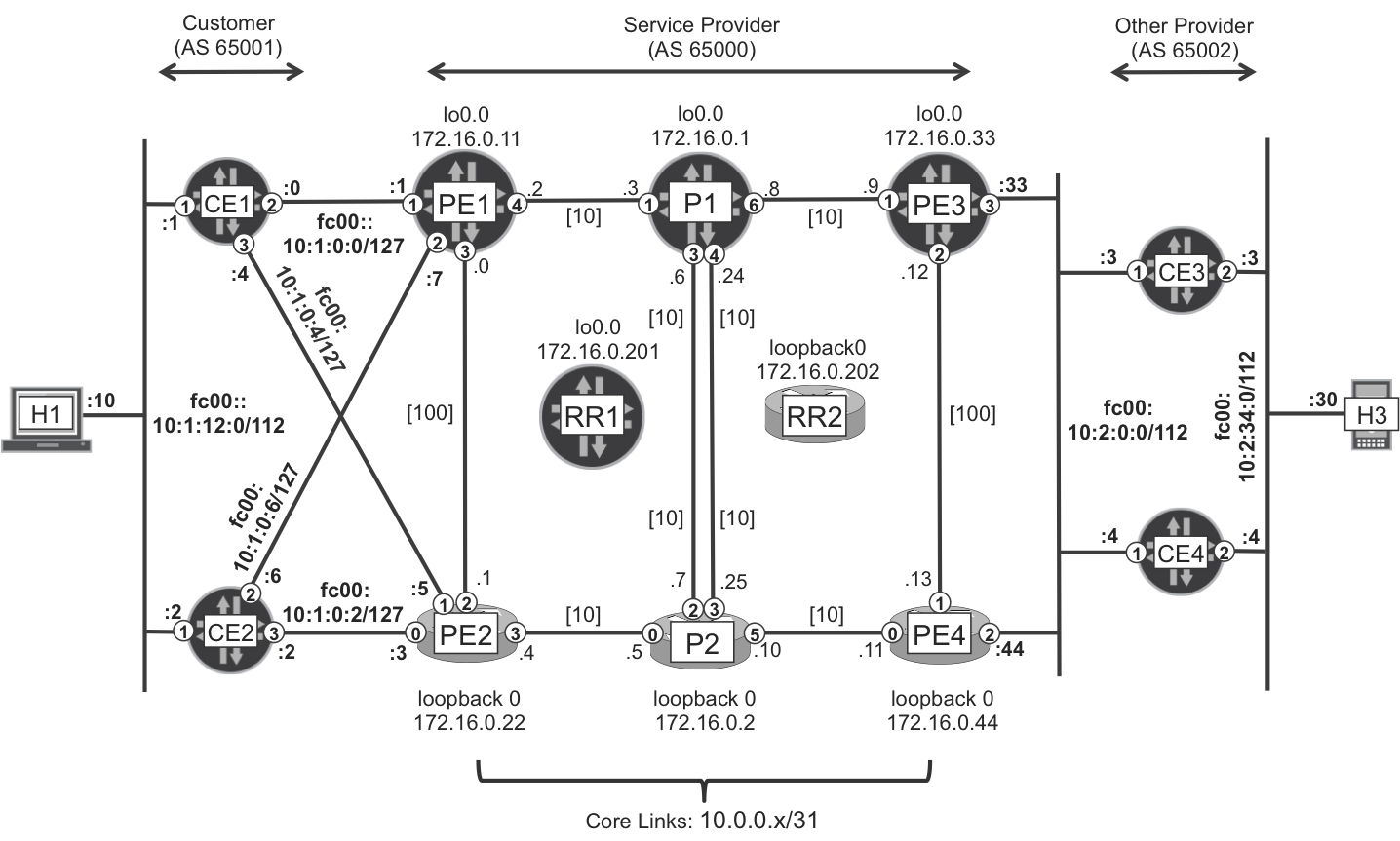
Figure 3-1. 6PE Topology
Note
From now on, in Chapter 3 through Chapter 9, the PE1-PE2 and PE3-PE4 links have Intermediate System–to–Intermediate System (IS-IS) metric 100. So, the preferred path from PE1 to PE4 is PE1-P1=P2-PE4, and vice versa.
The hosts, CEs, and PEs, are dual-stack devices that support both IPv4 and IPv6. To make the example easy to follow, IPv6 addressing looks very similar to IPv4. For example, H1 has IPv4 and IPv6 addresses 10.1.12.10/24 and fc00:0:0:0:10:1:12:10/112, respectively. Shortened with the “::” construct—which means all zeros and can only appear at most once in an IPv6 prefix—thus, H1’s IPv6 address becomes fc00::10:1:12:10/112. Although the addresses look similar, the IPv4 and IPv6 prefixes are in decimal and hexadecimal format, respectively. So, this addressing choice is more cosmetic rather than a real translation of the bits from IPv4 to IPv6. And the example’s IPv6 mask /112 provides twice as many host bits than the IPv4 mask /24.
H1 has a default IPv6 route (0::0/0) pointing to fc00::10:1:12:100, a Virtual Router Redundancy Protocol (VRRP) group address whose default master is CE1. VRRP route tracking is in place, so if CE1 does not have visibility of the fc00::10:2:34:0/112 remote route but CE2 does, CE2 becomes the VRRP master.
Similarly, H3 has a default IPv6 route pointing to fc00::10:2:134:100, a VRRP group address whose master is CE4, provided that it has visibility of the fc00::10:1:12:0/112 remote route.
How about the IPv6 route exchange all the way between CE1 and CE4? Let’s go step by step, starting with the iBGP sessions between PEs and Route Reflectors (RRs).
6PE—Backbone Configuration at the PEs
Let’s see the configuration in Junos and IOS XR.
6PE—backbone configuration at Junos PEs
Example 3-1 shows the relevant core-facing configuration at PE1.
Example 3-1. 6PE—core-facing configuration at PE1 (Junos)
1     protocols {
2         mpls {
3             ipv6-tunneling;
4         }
5         bgp {
6             group iBGP-RR {
7                 family inet6 {
8                     labeled-unicast;
9     }}}}
So it looks like IPv6 packets are to be tunneled in MPLS (line 3). The internal BGP (iBGP) sessions convey IPv6 Labeled Unicast (AFI=2, SAFI=4) prefixes, instead of unlabeled IPv6 Unicast (AFI=2, SAFI=1) ones. You’ll see more about this in the signaling section.
6PE—backbone configuration at IOS XR PEs
Here is the relevant core-facing configuration at PE2:
Example 3-2. 6PE—core-facing configuration at PE2 (IOS XR)
1     router bgp 65000
2      address-family ipv6 unicast
3       allocate-label all
4      !
5      neighbor-group RR
6       address-family ipv6 labeled-unicast
7     !
The principle is the same as in Junos. PE2 assigns MPLS labels to IPv6 prefixes, and this information is sent via iBGP to the RRs. In addition, PEs exchange unlabeled prefixes with CEs via eBGP. Later in the chapter, see Example 3-8, line 10.
6PE—RR Configuration
This is the additional configuration at RR1:
Example 3-3. 6PE—RR configuration at RR1 (Junos)
1     protocols {
2         bgp {
3             group CLIENTS {
4                 family inet6 labeled-unicast;
5     }}}
6     routing-options {
7         rib inet6.0 static route 0::0/0 discard;
8     }
An IPv6 (AFI=2) BGP route carries a BGP next-hop attribute with IPv6 format. But RR1 is not running any IPv6 routing protocols, so it cannot resolve the BGP next hop. This is why a default IPv6 route is configured in lines 6 through 7.
Example 3-4 shows the additional configuration at RR2.
Example 3-4. 6PE—RR configuration at RR2 (IOS XR)
router bgp 65000
 address-family ipv6 unicast
 !
 neighbor-group CLIENTS
  address-family ipv6 labeled-unicast
   route-reflector-client
!
IOS XR does not require any extra configuration to resolve the BGP next hop.
6PE—Access Configuration at the PEs
Let’s now focus on the CE-PE routing. The most scalable protocol is BGP, and there are two configuration options for the PE1-CE1 connection:
-
The first option requires two eBGP sessions. One eBGP session is established between the IPv4 endpoints (10.1.0.0-1) and exchanges IPv4 unicast (AFI=1, SAFI=1) prefixes; the other session is established between the IPv6 endpoints (fc00::10:1:0:0-1) and exchanges IPv6 unicast (AFI=2, SAFI=1) prefixes.
-
The second option relies on a single eBGP session established between the IPv4 endpoints (10.1.0.0-1). This multiprotocol eBGP session is able to signal both IPv4 unicast (AFI=1, SAFI=1) and IPv6 unicast (AFI=2, SAFI=1) prefixes.
Both options are valid, but the second one is more scalable; hence, it is used here.
6PE—access configuration at Junos PEs
Example 3-5 shows the access configuration at PE1. The only logical interface and eBGP session displayed correspond to the PE1-CE1 link.
Example 3-5. 6PE—access configuration at PE1 (Junos)
1     interfaces {
2         ge-2/0/1 {
3             unit 1001 {
4                 vlan-id 1001;
5                 family inet address 10.1.0.1/31;
6                 family inet6 address fc00::10:1:0:1/127;
7     }}}
8     protocols {
9         bgp {
10            group eBGP-65001 {
11                family inet unicast;
12                family inet6 unicast;
13                peer-as 65001;
14                neighbor 10.1.0.0 export PL-eBGP-CE1-OUT;
15    }}}
16    policy-options {
17        policy-statement PL-eBGP-CE1-OUT {
18            term BGP {
19                from protocol bgp;
20                then metric 100;
21            }
22            term IPv6 {
23                from family inet6;
24                then next-hop fc00::10:1:0:1;
25    }}}
As you can see, the logical interface is dual-stacked (lines 5 and 6). Both IPv4 and IPv6 unicast (lines 11 and 12) prefixes can be exchanged on top of one single eBGP session (line 14).
The BGP next-hop rewrite in line 24 is essential. Without it, PE1 would advertise IPv6 routes to CE1 in the format shown in Example 3-6.
Example 3-6. 6PE—IPv4-mapped IPv6 BGP next hop
juniper@PE1> show route advertising-protocol bgp 10.1.0.0 detail
             table inet6.0

* fc00::10:2:34:0/112 (2 entries, 1 announced)
     [...]
     Nexthop: ::ffff:10.1.0.1
In classical IPv6 notation, ::ffff:10.1.0.1 is ::ffff:0a01:0001. This is an IPv4-mapped IPv6 address, automatically derived from 10.1.0.1. But, the PE1-CE1 link is configured with IPv6 network fc00::10:1:0:0, which is totally different—watch out for hex colon versus decimal dot. Hence, the need for a BGP next-hop rewrite: without it, CE1 would not be able to resolve the BGP next hop. The same technique must be applied for prefixes announced by CE1 to PE1. Following is the next hop after the policy is applied.
Example 3-7. 6PE—rewritten IPv6 BGP next hop
juniper@PE1> show route advertising-protocol bgp 10.1.0.0 detail table inet6.0

* fc00::10:2:34:0/112 (2 entries, 1 announced)
     [...]
     Nexthop: fc00::10:1:0:1
As a more complex alternative, you can install the ::ffff:10.1.0.1/128 route into inet6.3, which is the auxiliary table to resolve BGP next hops in IPv6 format. This technique is illustrated in Chapter 9.
Note
In the remainder of this section, dual-stack is assumed. Even if not shown, all of the BGP sessions are also configured with family inet unicast (address-family ipv4 unicast).
6PE—access configuration at IOS XR PEs
Following is the access configuration at PE2. The only logical interface and eBGP session displayed correspond to the PE2-CE2 link.
Example 3-8. 6PE—access configuration at PE2 (IOS XR)
1     interface GigabitEthernet0/0/0/0.1001
2      ipv4 address 10.1.0.3 255.255.255.254
3      ipv6 address fc00::10:1:0:3/127
4      encapsulation dot1q 1001
5     !
6     router bgp 65000
7      address-family ipv6 unicast
8      neighbor 10.1.0.2
9       remote-as 65001
10      address-family ipv6 unicast
11       route-policy PL-eBGP-65001-IN in
12       route-policy PL-eBGP-CE2-OUT out
13    !
The principle is very similar to Junos, except that IOS XR PE2 automatically performs the BGP next-hop rewrite (to fc00::10:1:0:3) on its IPv6 advertisements to CE2.
The eBGP route policies (lines 11 and 12) basically pass all the prefixes (see Chapter 1).
6PE—Signaling
Figure 3-2 illustrates the entire signaling and forwarding logic. The labeled IPv6 route signaling always relies on BGP. As for the transport mechanism, you have the same flexibility as with any other MPLS service: it can be based either on IP tunnels or, better, on MPLS LSPs (static, LDP, RSVP, BGP IPv4-LU, or SPRING). This example uses LDP, but any other option is valid.
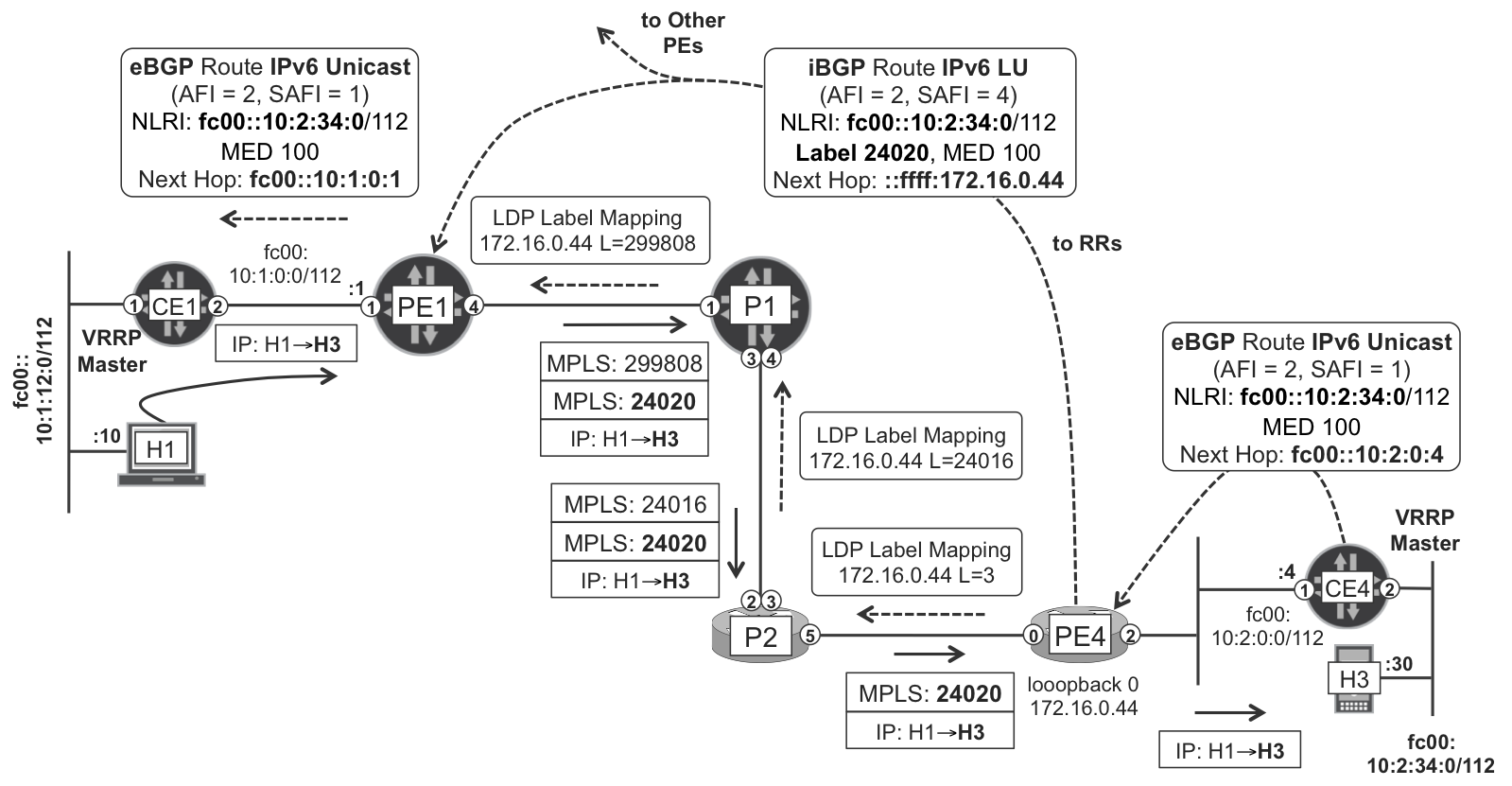
Figure 3-2. 6PE in action
Note
Refer back to Chapter 1 for an explanation as to why, in this multihoming scenario, the packet follows the path H1→CE1→PE1→...→PE4→CE4→H3.
Let’s first see the signaling flow. First, PE4 receives an IPv6 Unicast (AFI=2, SAFI=1) route from CE4, as shown in the following example:
Example 3-9. 6PE—IPv6 Labeled Unicast route
RP/0/0/CPU0:PE4# show bgp ipv6 unicast fc00::10:2:34:0/112
[...]
   Network    Next Hop        Metric LocPrf Weight Path
*> fc00::10:2:34:0/112
              fc00::10:2:0:4     100             0 65002 i
Then, PE4 allocates an MPLS label to the prefix and advertises it to the RRs. Example 3-10 shows how the IPv6 Labeled Unicast route advertised by PE4 looks from the perspective of RR1.
Example 3-10. 6PE—IPv6 Labeled Unicast route
1     juniper@RR1> show route receive-protocol bgp 172.16.0.44 detail table inet6.0
2
3     inet6.0: 3 destinations, 6 routes (...)
4     * fc00::10:2:34:0/112 (2 entries, 1 announced)
5          Accepted
6          Route Label: 24020
7          Nexthop: ::ffff:172.16.0.44
8          MED: 100
9         Localpref: 100
10         AS path: 65002 I
Note
RRs do not change the BGP next hop, and as a consequence they do not change the label encoded in the Network Layer Reachability Information (NLRI) either: the label is meaningful to the egress PE only.
You can refer to Example 3-7 to partially see the route advertised from PE1 to CE1.
6PE—Forwarding Plane
Let’s examine the forwarding bits illustrated in Figure 3-2 step by step. First, H1 sends the packet via its default gateway CE1, which holds the VRRP group’s virtual IPv6 and MAC addresses.
Next, CE1 must choose between two routes to the same destination: one from PE1 (with Multi Exit Discriminator [MED] 100), and another one from PE2 (with MED 200). CE1 chooses the best route, which is via PE1.
Then, PE1 looks at the BGP next hop of the Labeled Unicast route (Example 3-10, line 7), which is ::ffff:172.16.0.44. What does it mean? It is the IPv4-mapped IPv6 address derived from PE4’s IPv4 loopback address: 172.16.0.44.
Example 3-11. 6PE—BGP next-hop resolution at ingress PE—PE1 (Junos)
juniper@PE1> show route table inet6.3 ::ffff:172.16.0.44/128
[...]
::ffff:172.16.0.44/128
                   *[LDP/9] 2d 20:39:37, metric 30
                    > to 10.0.0.3 via ge-2/0/4.0, Push 299808
If you look back at Figure 3-2, you can see that P1 only advertises an LDP label mapping for the IPv4 FEC 172.16.0.44, not for ::ffff:172.16.0.44. Indeed, only the PEs are assumed to be IPv6-aware, and LDP only signals IPv4 FECs. In other words, there is no change at the LDP level when the 6PE service is turned on.
As you can see in Example 3-12, and in Figure 3-2, PE1 pushes two MPLS labels before sending the packet to P1.
Example 3-12. 6PE—Double MPLS label push at the ingress PE—PE1 (Junos)
1     juniper@PE1> show route forwarding-table destination fc00::10:2:34:0
2     [...]
3     Destination      Next hop   Type  Index    NhRef
4     fc00::10:2:34:0/112          indr  1048574      2
5                      10.0.0.3   Push 24020, Push 299808(top) ge-2/0/4.0
This is the first time that this book shows a double MPLS label push operation. There are several use cases for MPLS label stacking, and this is one of the most common: a bottom service label (24020 in line 5) and a top transport label (299808 in line 5). The transport label typically changes hop by hop, and in this example, it is eventually popped at the penultimate hop. On the other hand, the service label travels intact down to the egress PE, in this case PE4. And PE4 is the router that in the first instance had allocated that service label to the IPv6 prefix, so it knows how to interpret it.
Example 3-13. 6PE—MPLS label pop at the egress PE—PE4 (IOS XR)
1     RP/0/0/CPU0:PE4#show mpls forwarding
2     Local  Outgoing    Prefix
3     Label  Label       or ID
4     ------ ----------- ------------------
5     24020  Unlabelled  fc00::10:2:34:0/112
6
7     Outgoing        Next                        Bytes
8     Interface       Hop                         Switched
9     --------------  ------------------------    --------
10    Gi0/0/0/2.1001  fe80::205:8603:e971:f501    32576
When PE4 receives a packet with label 24020, it pops all the labels and sends the packet out toward CE4. How do you check that this strange IPv6 address in line 10 actually belongs to CE4? Let’s see how by taking a look at Example 3-14.
Example 3-14. 6PE—IPv6 link-local address
juniper@CE4> show interfaces ge-0/0/1.1001 terse
Interface      Admin Link Proto    Local
ge-0/0/1.1001  up    up   inet     10.2.0.4/24
                          inet6    fc00::10:2:0:4/112
                                   fe80::205:8603:e971:f501/64
Indeed, CE4 computes a link-local IPv6 address from the link’s MAC address.
6PE—why is there a service label?
PE4 pops the service label and maps the packet to the Internet Global IPv6 Routing Table. Does PE4 really need the service label? Not really. If PE4 had received a native IPv6 packet on its core uplink Gi 0/0/0/0, it would still have mapped the packet to the global routing table. And it would know that it is an IPv6 packet due to the Layer 2 (L2) header’s Ethertype, not to mention that the first nibble (four bits) of the packet is 6.
So, why is there a service MPLS label? The main reason is PHP. The 6PE model was developed assuming that no LSR (including the penultimate one) supports IPv6 on its core uplinks. If PE1 had only pushed the transport MPLS label, this would be the Bottom of Stack (BoS) label. After popping it, P2 inspects the resulting packet and finds a first nibble with value 6. This is definitely not an IPv4 packet, whose first nibble would be 4. So far, no problem: P2 should be able to send the packet to the egress PE (PE4), as dictated by the LSP. But there is one snag: after all this popping, the packet has no L2 header.
In IPv4, the solution is easy: P2 builds an L2 header with Ethertype 0x0800 (IPv4) and a destination MAC address corresponding to PE4—and resolved via Address Resolution Protocol (ARP) by asking who has 10.0.0.11.
Now, in IPv6, P2 needs to push an L2 header with Ethertype 0x86DD (IPv6), but to which destination MAC address? ARP is an IPv4 thing! In IPv6 you need Neighbor Discovery (ND), an ICMPv6 mechanism that relies on IPv6 forwarding. And this is not possible if P2 does not support or is not configured for IPv6.
By using a service label, things are made easier for P2 because there is still an MPLS label after popping the transport label. P2 builds the L2 header with Ethertype 0x8847 (MPLS) and the destination MAC address is the one resolved via ARP for 10.0.0.11.
OK, this is why there is a service label. But how important is its value if the egress PE is going to pop it anyway? This is where it becomes more interesting.
6PE—service label allocation
There are three service label allocation modes at the egress PEs:
- Per-prefix mode
- This is the default mode in IOS XR for routes learned from (or pointing to) CEs. Every different service prefix (in this case, IPv6 route) has a different label. This mode is illustrated in Figure 3-2.
- Per-CE
- Also called per-NH (next hop) mode. This is the default mode in Junos. Let’s illustrate it with an example. Imagine PE3 has 1,000 IPv6 routes pointing to CE3, and 500 IPv6 routes pointing to CE4. PE3 assigns two labels: L1 to the first 1,000 routes, and L2 to the other 500 routes.
- Per-table
- Also called per-VRF (even if strictly speaking in the 6PE case there is no VRF). An egress PE assigns the same label to all the prefixes in the same table.
The most scalable model is per-table, followed by per-CE. Why? Because the lower the number of labels, the lower the number of forwarding next hops that the remote ingress PEs need to store and update.
However, using a high number of labels has an advantage if the backbone is composed of LSRs that do not have the capability of extracting fields from the IPv6 payload to compute the load-balancing hash. Most of the modern platforms are capable of doing it; hence, the trend is toward reducing the number of labels.
Following is the procedure to tune IOS XR in order to use per-CE or per-VRF mode.
Example 3-15. 6PE—changing the label allocation mode in IOS XR
RP/0/0/CPU0:PE4#configure
RP/0/0/CPU0:PE4(config)#router bgp 65000
RP/0/0/CPU0:PE4(config-bgp)#address-family ipv6 unicast
RP/0/0/CPU0:PE4(config-bgp-af)#label mode ?
  per-ce        Set per CE label mode
  per-vrf       Set per VRF label mode
  route-policy  Use a route policy to select prefixes ...
The per-vrf mode is very interesting. The assigned label to all the global IPv6 prefixes is number 2 or, in other words, the IPv6 Explicit Null label. For this reason, it is recommended to turn on this mode in Junos, as follows:
Example 3-16. 6PE—per-table label allocation mode in Junos
protocols {
    bgp {
        group iBGP-RR {
            family inet6 labeled-unicast explicit-null;
}}}
Note
Using one label mode or another is a purely local decision. It is possible to have an interoperable network with PEs using different modes.
The choice of a label allocation mode has additional implications. The following statements hold true for Junos and might apply to IOS XR, too:
-
With per-prefix and per-CE modes, the egress PE performs an MPLS lookup on the packet, and as a result, the forwarding next hop is already determined. The egress PE is actually performing packet switching, in MPLS terms.
-
With per-table mode, the egress PE performs an IPv4 lookup on the packet after the MPLS label is popped. This results in a richer functionality set.
Now consider the PE-CE subnet fc00::10:2:0:0/112, which is local from the perspective of PE3. If PE3 is using per-CE mode for the 6PE service, what CE is actually linked to that prefix? Is it CE3 or CE4? Actually it’s neither. This is why, in per-CE mode, the local multipoint subnets are not advertised in Junos. You can still advertise CE3 (fc00::10:2:0:3/128) and CE4 (fc00::10:2:0:4/128) host routes if you locally configure a static route to the host.
6PE—traceroute
Here is a working traceroute from H1 (a host running IOS XR) to H3. You can compare the following example to Figure 3-2.
Example 3-17. 6PE—traceroute
RP/0/0/CPU0:H#traceroute fc00::10:2:34:30

 1  fc00::10:1:12:1 0 msec 0 msec 0 msec                   # CE1
 2  fc00::10:1:0:1 59 msec 9 msec 0 msec                   # PE1
 3  fc00::10:0:0:3 [MPLS: Labels 299808/24020 Exp 0] ...   # P1
 4  ::ffff:172.16.0.2 [MPLS: Labels 24016/24020 Exp 0] ... # P2
 5  fc00::10:2:0:44 0 msec 0 msec 39 msec                  # PE4
 6  fc00::10:2:0:4 39 msec 0 msec 0 msec                   # CE4
 7  fc00::10:2:34:30 0 msec 0 msec 9 msec                  # H4
The traceroute mechanism in an MPLS core is the same as the one described in Chapter 1 for IPv4 over MPLS packets. When an IPv6 packet’s Time-to-Live (TTL) expires at a transit LSR, such as P1 or P2, the LSR generates an ICMPv6 time exceeded toward the original source (H1). The resulting ICMPv6 message is then encapsulated on the original LSP (→PE4), so the egress PE (PE4) can IPv6-route it toward the source (H1) The egress PE (PE4) is configured in per-VRF label allocation mode, so it does not include the service label in the time exceeded message.
But how can a non-IPv6 LSR generate an ICMPv6 packet? IOS XR does it automatically by sourcing the packet from the IPv6 address that is mapped from its own loopback IPv4 address (line 4). As for Junos, it requires that you configure icmp-tunneling, and also some IPv6 addressing in place. The common practice is to configure IPv6 addresses on all the core links, and not to advertise them in the Interior Gateway Protocol (IGP)— in IS-IS, protocols isis no-ipv6-routing.
BGP/MPLS IP Virtual Private Networks
BGP/MPLS IP Virtual Private Networks (VPNs), often called L3VPNs, are the most popular application of MPLS. If someone enters a room full of network engineers and asks them to write down the first MPLS application that comes to mind, most will put L3VPN. That having been said, L3VPNs are not the leading MPLS service in terms of traffic. Instead, the classic Internet over MPLS service (Global IPv4 over MPLS) described in Chapter 1 transports the majority of the data and multimedia traffic in the world.
So why are L3VPNs so recognizable?
-
L3VPNs make it possible for customers to interconnect their headquarters, branch offices, and mobile users in a very simple manner. The Enterprises can keep their original private IP addressing, while the SP maintains the routing and traffic separate among tenants. In this way, connectivity and security needs are all addressed at the same time.
-
SPs achieve higher revenue per user (and per bit) compared to residential IP services.
True, there are other popular VPN technologies such as Secure VPNs based on IPsec or on SSL/TLS. These deal with similar business requirements and can even work over a plain Internet connection. But the flexibility, scalability, manageability, and simplicity of BGP/MPLS IP VPNs, both from the point of view of the tenant and of the SP, are unparalleled. BGP/MPLS IP VPNs remain an undeniably fundamental piece of the VPN portfolio in the world.
BGP/MPLS IP VPNs were originally described in RFC 2547, which was later obsoleted by RFC 4364. You can find a great description of this technology in the RFC itself:
This method uses a “peer model,” in which the customers’ edge (CE) routers send their routes to the Service Provider’s edge (PE) routers [...] Routes from different VPNs remain distinct and separate, even if two VPNs have an overlapping address space [...]. The CE routers do not peer with each other; hence, the “overlay” is not visible to the VPN’s routing algorithm [...].
In this book, the terms BGP/MPLS IP VPN and L3VPN are used interchangeably. This is not totally accurate because L3VPN also includes non-IP services such as OSI VPNs. However, for the sake of simplicity and readability we will use the term L3VPN. This section focuses on a dual stack (IPv4 and IPv6) scenario.
Attachment Circuits and Access Virtualization
Multiplexing at L2 is one of the primary forms of virtualization. For example, it is perfectly possible for one single CE-facing physical interface (such as PE1’s ge-2/0/1) to have several logical interfaces, each with its own VLAN/802.1q identifier. Each VLAN ID identifies a separate attachment circuit (AC), using the terminology of RFC 4364. An AC connects a PE either to a single CE or to a multipoint access network—such as an Ethernet Metropolitan Area Network (MAN).
The terminology can be a bit confusing across vendors. If you have some hands-on experience with Juniper and Cisco, you should certainly have noticed that an untagged Ethernet interface is directly configured in IOS XR, whereas in Junos it is done via unit 0. The reason lies in the following implementation difference:
-
In Junos, a physical interface (IFD: Interface Device) can have several logical interfaces (IFL: Interface Logical or unit), thanks to L2 multiplexing techniques such as VLAN tagging. On the other hand, if the IFD has a native encapsulation with no multiplexing, only one IFL is supported and it must be unit 0. In all cases, an AC in Junos is a CE-facing IFL.
-
In IOS XR, there are two options: an AC can be either a native (nonmultiplexed) physical interface, or if there is L2 multiplexing, a subinterface (similar to an IFL).
Note
Junos ACs are typically IFLs, whereas in IOS XR an AC can be a subinterface or an interface—depending on the encapsulation.
An AC is a logical concept. In L3 services, the AC is where service L3 parameters such as IP addresses are configured at the PE.
An AC is typically associated with a single service at the PE. Let’s use an example wherein PE1’s ge-2/0/1 has four IFLs with VLAN ID 1001, 1002, 1003, and 1004, respectively. The per-IFL unit number may match the VLAN ID or not—for simplicity, let’s suppose that it does match. It is perfectly possible to map IFL 1001 to a global Internet service, IFL 1002 to L3VPN A, IFL 1003 to L3VPN B, and IFL 1004 to an L2VPN.
On the other hand, one service can have several ACs at a given PE. For example, a PE can have several ACs connected to different CEs in such a way that all these ACs are associated to a global Internet service, or all of them to the same VPN.
AC classification—per technology
One of the most common AC types is VLAN-tagged Ethernet. One VLAN/802.1q header contains a 12-bit VLAN ID field, so its maximum value is 4,095. It’s also possible to stack two VLAN/802.1q headers inside the original MAC header, overcoming the limit of 4,096 VLANs in one LAN. This is a popular technique that has different names: stacked VLAN, Q-in-Q, SVLAN/CVLAN (where S stands for Service and C for Customer), and so on. VXLAN is a different technology, and it is discussed in Chapter 8.
In addition to the classic AC types (native Ethernet, VLAN-tagged Ethernet, ATM, Frame Relay, etc.), there are many other flavors. For example, an AC can actually be totally virtual, such as a VLAN transported in a locally terminated MPLS Pseudowire (see PWHE at Chapter 6), or a PPPoE session, or an L2TP session, or a dynamic interface created upon the headers of incoming IP traffic (IP demux), and so forth. Even an IPsec tunnel coming from the Internet can be terminated at the PE, itself becoming an AC of a BGP/MPLS IP VPN. Not all these access flavors are covered here, but there is an important concept to keep in mind: any connection with an endpoint at the PE can be a valid attachment circuit.
Going back to the classic ACs (such as basic Ethernet with or without VLANs), in many real-life scenarios the connection between CE and PE is not direct. An L2 service provider is typically in the middle, transporting the frames between CE and PE in a transparent manner—via either a point-to-point or a multipoint mechanism. In that case, the L2 carrier provides an overlay: the CEs and PEs are the only IP endpoints of the circuit connection. So, if the AC is Ethernet-based and the service is a BGP/MPLS IPv4 VPN, CE1 and PE1 can resolve each other’s IPv4 addresses by using ARP.
L3VPN in a Nutshell
In the examples that follow, the topology and IPv4/IPv6 addressing scheme remain the same as in Figure 1-1 and Figure 3-1, with the following differences:
-
The VLAN ID of the ACs is 1002 instead of 1001.
-
At the PEs, the ACs do not belong to the global routing instance, but to private instances called Virtual Routing and Forwarding (VRFs).
-
The PEs are the same, but a new set of CEs is used, one per site and VPN. For example, on the lefthand side, there is CE1-A and CE2-A for VPN A.
-
This is an Intranet VPN service, so CE3 (BR3) and CE4 (BR4) are replaced with CE3-A and CE4-A, respectively. The righthand AS is 65001, matching the lefthand AS number.
The primary goal of an MPLS VPN is to provide connectivity between tenant CEs that are attached to different PEs. The VPN concept is global, whereas a VRF is a local instance at a specific PE.
Note
For the time being, you can think of a VRF as the local representation of one (and only one) VPN. This will change later on in this chapter.
Many routing flavors and protocols (static routes, Routing Information Protocol [RIP], OSPF, IS-IS, eBGP) can run between CE and PE. We use eBGP in this book because it’s the most scalable protocol:
-
PE-CE eBGP sessions are used to exchange IP Unicast (SAFI=1) prefixes.
-
PE-RR iBGP sessions convey IP Unicast VPN (SAFI=128) prefixes.
How about the AFI? It’s 1 for IPv4; 2 for IPv6. So, for example, IPv6 VPN Unicast corresponds to [AFI=2, SAFI=128].
Note
IPv6 Unicast VPN is commonly called 6vPE
IP VPN prefixes have one thing in common with the Labeled Unicast (LU) prefixes used in the 6PE solution: they both encode a label in the NLRI. However, IP VPN is more complex because it also must provide information about the private context. This is achieved with the help of Route Distinguishers and Route Targets.
Given this, it’s only logical that L3VPN configurations are longer than 6PE’s. So let’s see L3VPN signaling and forwarding first; then, when the service is understood, move on to the configurations.
L3VPN—Signaling
Figure 3-3 illustrates the entire signaling and forwarding flow for IPv4 Unicast VPN. The IP VPN route signaling always relies on BGP. As for the transport mechanism, you have the same flexibility as with any other MPLS service: it can be based either on IP tunnels or, better, on MPLS LSPs (static, LDP, RSVP, BGP IPv4-LU, or SPRING). This example uses LDP, but any other option is valid.
Figure 3-3. IPv4 VPN Unicast in action
Note
Go to Chapter 1 for an explanation as to why, in this multihoming scenario, the packet follows the path H1→CE1A→PE1→...→PE4→CE4A→H3.
Let’s analyze the signaling flow for IPv4 and IPv6 prefixes. First, PE4 receives IPv4 Unicast and IPv6 Unicast routes from CE4-A.
Example 3-18. eBGP IPv4 and IPv6 Unicast routes
RP/0/0/CPU0:PE4# show bgp vrf VRF-A ipv4 unicast
[...]
   Network    Next Hop        Metric LocPrf Weight Path
*> 10.2.34.0/24
              10.2.0.4        100             0 65001 i

RP/0/0/CPU0:PE4# show bgp vrf VRF-A ipv6 unicast
[...]
   Network    Next Hop        Metric LocPrf Weight Path
*> fc00::10:2:34:0/112
              fc00::10:2:0:4     100             0 65001 i
Then, PE4 allocates an MPLS label to each prefix and advertises them to the RRs. Example 3-19 shows how the IPv4 Unicast VPN and IPv6 Unicast VPN routes advertised by PE4 look, from the perspective of RR1.
Example 3-19. L3VPN—IPv4 and IPv6 Unicast VPN routes (Junos)
1     juniper@RR1> show route receive-protocol bgp 172.16.0.44 detail
2                  table bgp.l3vpn
3
4     bgp.l3vpn.0: 6 destinations, 12 routes [...]
5     * 172.16.0.44:101:10.2.34.0/24 [...]
6          Accepted
7          Route Distinguisher: 172.16.0.44:101
8          VPN Label: 24022
9          Nexthop: 172.16.0.44
10         MED: 100
11         Localpref: 100
12         AS path: 65001 I
13         Communities: target:65000:1001
14
15    bgp.l3vpn-inet6.0: 6 destinations, 12 routes [...]
16
17    * 172.16.0.44:101:fc00::10:2:34:0/112 [...]
18         Accepted
19         Route Distinguisher: 172.16.0.44:101
20         VPN Label: 24023
21         Nexthop: ::ffff:172.16.0.44
22         MED: 100
23         Localpref: 100
24         AS path: 65001 I
25         Communities: target:65000:1001
Note
Remember that RRs do not change the BGP next-hop attribute by default. For this reason, they do not change the VPN label, either.
Example 3-20 shows these same routes from the perspective of PE4 itself.
Example 3-20. L3VPN—IPv4 and IPv6 Unicast VPN routes (IOS XR)
RP/0/0/CPU0:PE4#show bgp vpnv4 unicast advertised
Route Distinguisher: 172.16.0.44:101
10.2.34.0/24 is advertised to 172.16.0.201 [...]
  Attributes after outbound policy was applied:
    next hop: 172.16.0.44
    MET ORG AS EXTCOMM
    origin: IGP  neighbor as: 65001  metric: 100
    aspath: 65001
    extended community: RT:65000:1001
    /* Same route advertised to RR2 (omitted) */

RP/0/0/CPU0:PE4#show bgp vpnv6 unicast advertised
Route Distinguisher: 172.16.0.44:101
fc00::10:2:34:0/112 is advertised to 172.16.0.201 [...]
  Attributes after outbound policy was applied:
    next hop: 172.16.0.44
    MET ORG AS EXTCOMM
    origin: IGP  neighbor as: 65001  metric: 100
    aspath: 65001
    extended community: RT:65000:1001
    /* Same route advertised to RR2 (omitted) */
Example 3-19 and Example 3-20 also introduced three key L3VPN concepts: Route Distinguisher, VPN Label, and Route Target.
Route Distinguisher
Route Distinguisher (RD) is a very accurate name. An RD does precisely what the term implies: it distinguishes routes. PE4 may have the route 10.2.34.0/24 in different VRFs. The host 10.2.34.30 may be a server in a multinational enterprise (VRF-A), and at the same time a mobile terminal in a university (VRF-B). VPNs provide independent addressing spaces, so prefixes from different VRFs can overlap with no collision.
The prefixes exchanged over PE-CE eBGP sessions are IP Unicast (SAFI=1) and they do not contain any RDs. Indeed, from the point of view of the PE, each eBGP session is bound to one single VRF, so there is no need to distinguish the prefixes. On the other hand, CEs have no VPN awareness: from the perspective of the CE, a PE is just an IPv4/IPv6 router.
Now, one single PE-RR (or PE-PE) iBGP session can signal prefixes from multiple VPNs. For example, PE4 may advertise the 10.2.34.0/24 route from VRF-A and VRF-B. The 10.2.34.0/24 prefix represents a different reality in each of the VRFs, and this is where an RD comes in handy. The actual prefixes that PE4 announces to the RRs are <RD1>:10.2.34.0/24 and <RD2>:10.2.34.0/24. These prefixes are different as long as <RD1> is different from <RD2>.
Note
In a given PE, you must configure each VRF with a different RD. It is also possible to configure a router so that it automatically generates a distinct RD for each VRF.
Back in Figure 3-3, the RD is 172.16.0.44:101. There are several ways to encode RDs, as regulated by IANA. This book discusses two types: 0 and 1. These formats are <AS>:<VPN_ID> and <ROUTER_ID>:<VPN_ID>, respectively.
In an Active-Backup redundancy scheme, CE3-A and CE4-A advertise the 10.2.34.0/24 prefix with a different MED: 200 to PE3 and 100 to PE4, respectively. This makes PE3 prefer the iBGP route over the eBGP route; as a result, PE4 does not advertise it to the RRs. In this model, the RD choice is not very important.
In an Active-Active redundancy scheme, CE3-A and CE4-A would advertise the 10.2.34.0/24 with the same MED, so both PE3 and PE4 would in turn advertise it to the RRs. In this case, the RD choice is critical. Let’s consider the case of VRF-A:
-
If the RD format is
<AS>:<VPN_ID>, unless each PE assigns a different<VPN_ID>to the VRF—which would result in a virtually unmanageable numbering scheme—both PE3 and PE4 advertise the 65000:101:10.2.34.0/24 prefix. The RR selects the best route (from its point of view) and reflects it. This results in information loss and suboptimal routing. Not only that, it also causes a delay in failure recovery. The RRs must detect that the primary route is not valid before they can advertise the backup route to the ingress PEs. Typically, RRs have many peers, so this process usually takes time, and RRs act as a control-plane bottleneck. In the Internet service, BGP Add-Path extensions were required to address this challenge, but not necessarily in IP VPN, where there is a native solution! -
If the RD format is
<ROUTER_ID>:<VPN_ID>, PE3 and PE4 advertise two different prefixes: 172.16.0.33:101:10.2.34.0/24 and 172.16.0.44:101:10.2.34.0/24, respectively. These are two different NLRI prefixes, and RRs reflect both of them. This guarantees that all of the PEs have all the information, achieving optimal routing and improved convergence. This is the scheme we use in this book. Note that in this case the<VPN_ID>value is the same (101) on both PEs, but this is not mandatory.
It is possible to have iBGP multihoming with unequal-cost multipath—see Chapter 20 for more details. The ingress PE can load-balance traffic between several egress PEs, even if these are not at the same IGP distance.
VPN label
The VPN label is an MPLS label that is locally significant to the egress PE. It is a service label by which the egress PE can map the downstream (from the core) user packets to the appropriate VRF (or CE). Like in 6PE, there are different label allocation schemes, which we’ll discuss later.
Although the VPN label is encoded in the IP Unicast VPN (SAFI=128) NLRI, routers in general—and RRs in particular—consider it more like a route attribute rather than as part of the NLRI. In other words, two identical RD:route prefixes are considered to be the same even if the VPN label is different. Thus, the RRs only reflect one of them.
Note
RRs do not change the BGP next hop, and as a consequence they do not change the label encoded in the NLRI either: the label is meaningful to the egress PE only.
Route Target
The Route Target (RT) concept is probably the one that makes BGP/MPLS VPNs so powerful. RTs are one type of BGP extended community.
Note
You can see an exhaustive list of standard Extended Communities in RFC 7153 and at http://www.iana.org/assignments/bgp-extended-communities/bgp-extended-communities.txt.
Every BGP VPN route carries at least one RT. RTs control the distribution of VPN routes. How? Locally at a PE, a VRF has the following export and import policies:
-
An export policy influences the transition of (local and CE-pointing) VRF routes from IP Unicast to IP Unicast VPN, before these routes are advertised to the RRs or other PEs. The export policy can filter prefixes and change their attributes; its most important task is to add RTs to the IP Unicast VPN routes.
-
An import policy influences the installation of remote IP Unicast VPN routes into the local VRFs. The import policy can filter prefixes and change their attributes; its most important task is to look at the incoming routes’ RTs and make a decision as to whether to install the route on the VRF where the import policy is applied.
You could view RTs as door keys. When a PE advertises a VPN route, it adds a key chain to the route. When the route arrives to other PEs, the route’s keys (RTs) can open one or more doors (import policies) at the target PE. These doors give access to rooms (VRFs) where the route is installed after stripping the RD.
For example, you can configure VRF-A on all PEs to export RT 65000:1001 and to also import RT 65000:1001. This symmetrical policy—with the same import and export RT—results in a full-mesh topology in which all the CEs are reachable from one another. In this sense, you can easily identify VPN A routes: they all carry RT 65000:1001.
But there are many other ways to configure RT policies (hub-and-spoke, service chaining, etc.). Indeed, RTs are a fundamental concept that will be discussed quite a few times in this book. Let’s move on.
L3VPN—Forwarding Plane
This section takes a look at the forwarding bits back in Figure 3-3, step by step. The text will describe what happens to an IPv4 packet, but the command output also shows the IPv6 variant.
First, H1 sends the packet via its default gateway CE1-A, which holds the VRRP group’s virtual IPv4 and MAC addresses.
Next, CE1-A must choose between two routes to the same destination: one from PE1 (with MED 100) and another one from PE2 (with MED 200). CE1-A chooses the best route, which is via PE1.
Prior to forwarding the packet, PE1 must have installed the route to the destination in its forwarding table. To do that, PE1 first looks at the BGP next hop of the labeled unicast route (Example 3-19, line 9), which is 172.16.0.44. This BGP next hop is present in PE1’s inet.3 table, with a forwarding next hop that says push 299808 label, send to P1. PE1 combines this instruction with the VPN label (Example 3-19, line 8), so it pushes two MPLS labels before sending the packet to P1.
Example 3-21. L3VPN—double MPLS label push at ingress—PE1 (Junos)
1     juniper@PE1> show route forwarding-table destination 10.2.34.30
2                  table VRF-A
3     [...]
4     Destination      Next hop   Type  Index    NhRef
5     10.2.34.0/24                indr  1048587      2
6                      10.0.0.3   Push 24022, Push 299808(top) ge-2/0/4.0
7
8     juniper@PE1> show route forwarding-table destination fc00::10:2:34:0
9                  table VRF-A
10    [...]
11    Destination      Next hop   Type  Index    NhRef
12    fc00::10:2:34:0/112         indr  1048584      2
13                     10.0.0.3   Push 24023, Push 299808(top) ge-2/0/4.0
Note
In Junos, 6vPE (like 6PE) routes get their BGP next hop resolved in the auxillary table inet6.3.
There is a bottom service label (24022 in line 6) and a top transport label (299808 in line 6). The transport label typically changes hop by hop—in this example, it is popped at the penultimate hop. Conversely, the service label travels intact down to the egress PE—in this case PE4. And because PE4 is the router that in the first instance had allocated the service label to the IPv4 VPN prefix, it therefore knows how to interpret it fully.
Example 3-22. L3VPN—MPLS label pop at the egress PE—PE4 (IOS XR)
RP/0/0/CPU0:PE4#show mpls forwarding vrf VRF-A
Local  Outgoing    Prefix              Outgoing        Next    Bytes
Label  Label       or ID               Interface       Hop     Switched
------ ----------- ------------------  --------------  -----   -------
24022  Unlabelled  10.2.34.0/24[V]     Gi0/0/0/2.1001  10.2.0.4

Local  Outgoing    Prefix
Label  Label       or ID
------ ----------- ------------------
24023  Unlabelled  fc00::10:2:34:0/112[V]

Outgoing        Next                        Bytes
Interface       Hop                         Switched
--------------  ------------------------    --------
Gi0/0/0/2.1001  fe80::205:8603:e971:f501    0
Finally, it is interesting to see how the return route (to 10.1.12.0/24) looks from the perspective of PE4—acting as an ingress PE.
Example 3-23. L3VPN—double MPLS label push at ingress—PE4 (IOS XR)
RP/0/0/CPU0:PE4#show cef vrf VRF-A 10.1.12.0/24
10.1.12.0/24 [...]
   via 172.16.0.22, 5 dependencies, recursive [flags 0x6000]
    recursion-via-/32
    next hop VRF - 'default', table - 0xe0000000
    next hop 172.16.0.22 via 24005/0/21
     next hop 10.0.0.10/32 Gi0/0/0/0 labels imposed {24002 24019}
You can use the same command for IPv6 prefixes. In that case, ensure that you introduce the keyword ipv6 between the VRF name and the prefix.
L3VPN—Backbone Configuration at the PEs
Let’s take a look at the backbone configuration in Junos and IOS XR.
L3VPN—backbone configuration at Junos PEs
Example 3-24 shows the relevant core-facing configuration at PE1.
Example 3-24. L3VPN—core-facing configuration at PE1 (Junos)
protocols {
    bgp {
        group iBGP-RR {
            family inet-vpn unicast;
            family inet6-vpn unicast;
}}}
As expected, two new address families are added: IPv4 Unicast VPN (AFI=1, SAFI=128) and IPv6 Unicast VPN (AFI=2, SAFI=128).
Note
You must also configure IPv6 tunneling as shown in Example 3-1, line 3. This is needed in order to install IPv4-mapped addresses in the inet6.3 auxiliary table.
L3VPN—backbone configuration at IOS XR PEs
Here is the relevant core-facing configuration at PE2:
Example 3-25. L3VPN—core-facing configuration at PE2 (IOS XR)
router bgp 65000
 address-family vpnv4 unicast
 address-family vpnv6 unicast
 !
 neighbor-group iBGP-RR
  address-family vpnv4 unicast
  address-family vpnv6 unicast
!
Note
Regardless of the transport LSP technology you use, don’t forget to globally configure mpls ldp. Otherwise, IP VPN prefixes will remain unresolved in the Cisco Express Forwarding (CEF). If you do not really need LDP as a protocol, just configure mpls ldp without any interfaces below.
L3VPN—RR Configuration
Example 3-26 lays out the additional configuration at RR1.
Example 3-26. L3VPN—RR configuration at RR1 (Junos)
1     protocols {
2         bgp {
3             group CLIENTS {
4                 family inet-vpn unicast;
5                 family inet6-vpn unicast;
6     }}}
7     routing-options {
8         rib inet.3 static route 0/0 discard;
9         rib inet6.3 static route 0::0/0 discard;
10    }
Note
In the examples in this chapter, MPLS is fully functional and LDP is active at all the PE-PE, PE-P, and P-P links. However, the RRs have no MPLS configuration in place.
An IP VPN Unicast (SAFI=128) BGP route has a private context. Indeed, transit P-routers do not keep any IP VPN routing state. For this reason, packets matching such route must be transported to the egress PE via an IP tunnel or an MPLS LSP.
In Junos, the tables in which BGP next hops can be resolved into labeled paths are inet.3 (for IPv4) and inet6.3 (for IPv6). Because this example’s RRs do not run any MPLS protocol, they need static routes (lines 8 and 9) to perform BGP next-hop resolution and reflect IP VPN routes.
Following is the additional configuration at RR2:
Example 3-27. L3VPN—RR configuration at RR2 (IOS XR)
1     router bgp 65000
2      address-family vpnv4 unicast
3      address-family vpnv6 unicast
4      !
5      neighbor-group CLIENTS
6       address-family vpnv4 unicast
7        route-reflector-client
8       !
9       address-family vpnv6 unicast
10       route-reflector-client
11    !
IOS XR does not require any extra configuration to resolve the BGP next hop.
L3VPN—VRF Configuration at the PEs
Now, let’s take a look at the VRF configuration in Junos and IOS XR.
L3VPN—VRF configuration at Junos PEs
Example 3-28 presents the access configuration at PE1. The only logical interface and eBGP session displayed correspond to the PE1-CE1 link.
Example 3-28. L3VPN—VRF configuration at PE1 (Junos)
1     interfaces {
2         ge-2/0/1 {
3             unit 1002 {
4                 vlan-id 1002;
5                 family inet address 10.1.0.1/31;
6                 family inet6 address fc00::10:1:0:1/127;
7     }}}
8     routing-instances {
9         VRF-A {
10            instance-type vrf;
11            interface ge-2/0/1.1002;
12            route-distinguisher 172.16.0.11:101;
13            vrf-export PL-VRF-A-EXP;
14            vrf-import PL-VRF-A-IMP;
15            protocols {
16                bgp {
17                    group eBGP-65001 {
18                        family inet unicast;
19                        family inet6 unicast;
20                        peer-as 65001;
21                        as-override;
22                        neighbor 10.1.0.0 {
23                            export PL-VRF-A-eBGP-CE1A-OUT;
24                        }
25    }}}}}
26    policy-options {
27        policy-statement PL-VRF-A-eBGP-CE1A-OUT {
28            term BGP {
29                from protocol bgp;
30                then {
31                    metric 100;
32                    community delete RT-ALL;
33                }
34            }
35            term IPv6 {
36                from family inet6;
37                then {
38                    next-hop fc00::10:1:0:1;
39                }
40        }}
41        policy-statement PL-VRF-A-EXP {
42            term eBGP {
43                from protocol bgp;
44                then {
45                    community add RT-VPN-A;
46                    accept;
47                }
48        }}
49        policy-statement PL-VRF-A-IMP {
50            term VPN-A {
51                from community RT-VPN-A;
52                then accept;
53            }
54        }
55        community RT-ALL members target:*:*;
56        community RT-VPN-A members target:65000:1001;
57    }
The AC configuration (lines 1 through 6) has nothing special: just a dual-stack IFL.
The VRF export (lines 13, and 41 through 46) and VRF import (lines 14, and 49 through 52) are very simple, to the point that they would not need to be defined. You could replace lines 13 and 14 with vrf-target target:65000:1001. But this shortcut is compatible only with full-mesh VPN topologies, and it does not allow filtering or modifying prefixes. For this reason, it’s a good practice to use the syntax in Example 3-28.
The as-override configuration in line 21 is not specific to L3VPNs. In fact, it is required for any BGP-based design that requires connecting two islands with the same AS (65001 in this case). Otherwise, the AS-loop detection logic would drop the prefixes at some point. There are other techniques to achieve the same result, but this one is simple.
Unlike IOS XR, when Junos readvertises an IP Unicast VPN route—after converting it to IP Unicast format—it keeps all the communities, including the RTs. It is a good practice to strip the RTs before sending the route to a plain CE (line 32).
As for the IPv6 next-hop rewrite in line 38, it is due to the fact that there is a single eBGP session used for IPv4 and IPv6 prefixes. The rationale is the same as explained previously in the 6PE section. (See the full discussion with respect to Example 3-6.)
L3VPN—VRF configuration at IOS XR PEs
Example 3-29 contains the access configuration at PE4. The only logical interface and eBGP session displayed correspond to the PE4-CE4A link.
Example 3-29. L3VPN—VRF configuration at PE4 (IOS XR)
1     interface GigabitEthernet0/0/0/2.1002
2      vrf VRF-A
3      ipv4 address 10.2.0.44 255.255.255.0
4      ipv6 address fc00::10:2:0:44/112
5      encapsulation dot1q 1002
6     !
7     router bgp 65000
8      vrf VRF-A
9       rd 172.16.0.44:101
10      address-family ipv4 unicast
11      address-family ipv6 unicast
12      !
13      neighbor 10.2.0.4
14       remote-as 65001
15       address-family ipv4 unicast
16        route-policy PL-VRF-A-eBGP-CE4A-IN in
17        route-policy PL-VRF-A-eBGP-CE4A-OUT out
18        as-override
19       !
20       address-family ipv6 unicast
21        route-policy PL-VRF-A-eBGP-CE4A-IN in
22        route-policy PL-VRF-A-eBGP-CE4A-OUT out
23        as-override
24    !
25    vrf VRF-A
26     address-family ipv4 unicast
27      import route-target
28       65000:1001
29      export route-target
30       65000:1001
31     !
32     address-family ipv6 unicast
33      import route-target
34       65000:1001
35      export route-target
36       65000:1001
37    !
38    route-policy PL-VRF-A-eBGP-CE4A-IN
39      pass
40    end-policy
41    !
42    route-policy PL-VRF-A-eBGP-CE4A-OUT
43      pass
44    end-policy
Note
See the discussion about eBGP policies in Chapter 1. It explains why eBGP pass policies are required in IOS XR but not in Junos.
As a side note, there is one significant configuration difference in the way non-BGP prefixes can be announced via BGP. In Junos, you need to modify the VRF export policy. Here is the syntax in IOS XR: router bgp <AS> vrf <VRF> address-family <AF> redistribute [...].
L3VPN—Routing Tables in Junos
You have already seen a few auxiliary tables: inet.3 and inet6.3 are used to resolve BGP IPv4 and IPv6 next hops, respectively. Their routes never make it to the forwarding table.
On the other hand, the bgp.l3vpn.0 and bgp.l3vpn-inet6.0 tables store the received RD:IPv4 and RD:IPv6 prefixes, respectively. Only the prefixes that match a local VRF’s import policy—typically, because the route’s RTs matches the import policy’s RTs—are stored. The other prefixes are simply discarded by default.
There are several exceptions to this discard-if-no-match rule. First, is PEs with the keep all knob configured. Second, certain routers readvertise IP Unicast VPN routes in IP Unicast VPN (SAFI=128) format:
-
RRs readvertise IP VPN iBGP routes as IP VPN iBGP routes.
-
Inter-AS Option B ASBRs (a concept discussed in Chapter 9) readvertise IP VPN iBGP routes as IP VPN eBGP routes, and vice versa.
-
A variant of the latter involves eiBGP (confederations) instead of eBGP.
In all of these exceptions, the device installs all the incoming IP VPN routes in the bgp.l3vpn[-inet6].0 auxiliary tables.
Let’s forget for the moment about these exceptions and think of a regular PE that receives a matching route. After the RD is stripped from it, the IP prefix is copied—as a secondary route—to the VRFs with a matching import policy. Yes, there can be several matching VRFs, and that will be discussed later. In the case of VRF-A, IPv4 and IPv6 prefixes are stored in VRF-A.inet.0 and VRF-A.inet6.0 routing tables, respectively.
Note
Defining a VRF as a table has been cautiously avoided. In fact, a VRF is an instance that can have several tables, one for each route type.
As you can see in Figure 3-4, the export logic is a bit different from that of the import. In Junos, by default, IP Unicast VPN routes are advertised directly from the VRF, not from L3VPN auxiliary tables.
However, if a device reflects IP VPN prefixes (like RR1), or if you configure the advertise-from-main-vpn-tables knob, all the IP VPN routes are advertised from the bgp.l3vpn[-inet6].0 table. Let’s call it the main IP VPN table. Now suppose that RR1 is also a PE and it has a local VRF connected to CE10. RR1 installs IP VPN prefixes learned from CE10 into the VRF (primary RIB) and copies them into the main IP VPN table (secondary RIB). In this case, which is not shown in Figure 3-4, RR1 advertises all the prefixes (either reflected or originated in the VRF) from the main IP VPN table.
Figure 3-4. IPv4 Unicast VPN—Junos routing tables
Do you really need to worry about from which table the routes are exported? If, for whatever reason, a PE advertises IP Unicast VPN prefixes from the main IP VPN table, the BGP next hop of these routes cannot be changed with VRF export policies; you can do it only with the global export policy applied to the iBGP group. On a separate note, if the primary RIB of an advertised prefix is the local VRF, the global export policy applies to this prefix only if you configure vpn-apply-export under the group.
Virtual routers
The idea of having a private routing instance is very attractive, and not only in the context of an L3VPN service. For example, a physical CE can be turned into a set of virtual CEs, each with its own upstream circuits and routing table(s).
In Junos, this is called virtual router (VR, a.k.a., VRF Lite), and you can configure it as shown in Example 3-28, with the following differences:
-
The
instance-typein line 10 isvirtual-router. -
Lines 12 through 14 must be removed, and line 32 is not necessary.
Graphically, if you disconnect VRF-A.inet.0 from bgp.l3vpn.0 in Figure 3-4, VRF-A becomes a VR.
Note
You cannot further virtualize virtual routers. Conversely, Junos Logical Systems can in turn contain their own VRFs and VRs.
The Cisco term for this same concept is VRF Lite. You can turn VRF-A into a VRF Lite by suppressing lines 27 through 30, and 33 through 36 from Example 3-29. Note that eBGP configuration in VRF Lite requires that you configure an RD, even if it is not actually signaled.
L3VPN—Service Label Allocation
The three different label allocation modes are already described in the context of 6PE. The concepts are the same with L3VPN.
The default label allocation mode in IOS XR is per-prefix, but you can change it to per-CE or per-VRF mode, as demonstrated in the following example:
Example 3-30. L3VPN—changing the label allocation mode in IOS XR
RP/0/0/CPU0:PE4#configure
RP/0/0/CPU0:PE4(config)#router bgp 65000
RP/0/0/CPU0:PE4(config-bgp)#vrf VRF-A
RP/0/0/CPU0:PE4(config-bgp-vrf)#address-family ipv4 unicast
RP/0/0/CPU0:PE4(config-bgp-vrf-af)#label mode ?
  per-ce        Set per CE label mode
  per-vrf       Set per VRF label mode
  route-policy  Use a route policy to select prefixes ...
Note
IOS XR per-prefix mode is the default for routes learned from (or pointing to) CEs. Other VRF prefixes (directly connected, static to Null0, aggregate) are all advertised with the same label by default.
It is possible to do the same tuning for address-family ipv6 unicast. In any case, a label that is bound to an IPv4 prefix is never bound to an IPv6 prefix in IOS XR: different label sets are kept for each address family.
This is different in Junos, for which per VRF label allocation mode associates the same label to all the prefixes in a VRF, regardless of whether they are IPv4 or IPv6.
The default label allocation mode in Junos is per-CE, but you can change it to per-VRF in two different ways. Let’s look at the first one:
Example 3-31. 6PE—per-table label allocation mode in Junos (I)
routing-instances VRF-A vrf-table-label;
This configuration creates a Label-Switched Interface (LSI), which is a global virtual IFL that is associated to one single MPLS label and to one single VRF. This LSI processes all the downstream (from the core) packets with that MPLS label: the label is popped and the packet is mapped to the correct VRF.
Example 3-32 depicts the second method, which is mutually exclusive to the first one.
Example 3-32. 6PE—per-table label allocation mode in Junos (II)
1     chassis {
2         fpc 2 pic 0 tunnel-services bandwidth 10g;
3     }
4     interfaces {
5         vt-2/0/0 unit 101 family inet;
6     }
7     routing-instances {
1         VRF-A interface vt-2/0/0.101;
2     }
The result is similar to an LSI, but this time the virtual IFL is anchored to a specific Packet Forwarding Engine (PFE) in the PE. This results in lower resource consumption because the IFL (Virtual Tunnel or vt-) is only instantiated in one PFE. On the other hand, the placement of the tunnel resources must be carefully planned to achieve an optimal forwarding path inside the router. Finally, it is possible to provision redundant vt- interfaces for a higher resiliency.
In both Junos and IOS XR, it is possible to change the label allocation method in a granular manner with policies. You can select different methods for different VRFs, and even for different prefix sets inside the same VRF.
L3VPN—Topologies
Symmetric VRF import and export policies using one single (and distinct) RT per VRF results in a full-mesh routing topology. Any site can reach any other site in the VPN, but you can tune RT policies to create arbitrary routing topologies. This is not only true for L3VPN: it also applies to any BGP-based service.
L3VPN—hub-and-spoke VPN
The lefthand scenario in Figure 3-5 shows a classic hub-and-spoke L3VPN. PE1 and PE2 are the hub PEs, connected to the corporate headquarters’ data center. PE3 and PE4 are spoke PEs, connected to small offices, home offices, or mobile users.
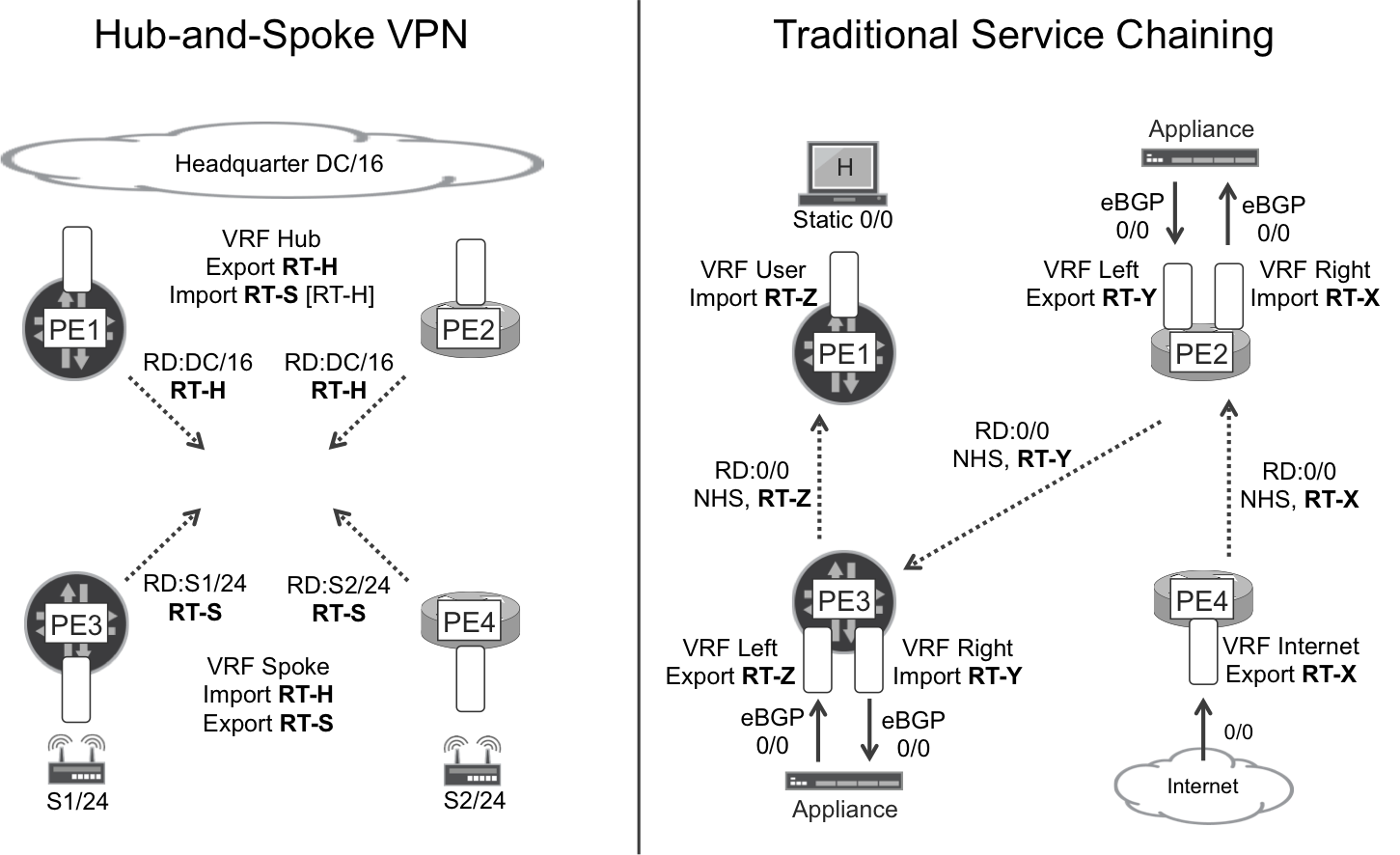
Figure 3-5. L3VPN Topology Samples
The remote sites do not need to communicate with one another.
With these connectivity requirements, hub-and-spoke PEs use complementary policies in the context of the same VPN:
-
Spoke PEs export routes with route target RT-S, so hub PEs import them.
-
Hub PEs export routes with route target RT-H, so spoke PEs import them.
-
Spoke PEs do not import routes from other spoke PEs.
-
Hub PEs may import routes from other hub PEs, if their import policies are configured to also accept routes with RT-H. This adds an extra level of redundancy.
The following example shows a typical asymmetrical RT configuration in Junos.
Example 3-33. L3VPN—hub VPN policy configuration (Junos)
1     policy-options {
2         policy-statement PL-VRF-A-HUB-EXP {
3             term eBGP {
4                 from protocol bgp;
5                 then {
6                     community add RT-VPN-A-HUB;
7                     accept;
8                 }
9         }}
10        policy-statement PL-VRF-A-HUB-IMP {
11            term VPN-A {
12                from community [ RT-VPN-A-SPOKE RT-VPN-A-HUB ];
13                then accept;
14            }
15        }
16        community RT-VPN-A-HUB members target:65000:2001;
17        community RT-VPN-A-SPOKE members target:65000:3001;
18    }
Junos applies the following logical operators:
- [OR]
- This operator is applied if several communities are listed in a
from communitystatement. It is enough for the route to contain any of the communities in order to match the term. - [AND]
- This operator is applied if several communities are listed in
members. The route must contain all the communities in order to match the community.
Following is an IOS XR sample.
Example 3-34. L3VPN—hub VPN configuration (IOS XR)
1     vrf VRF-A-HUB
2      address-family ipv4 unicast
3       import route-target
4        65000:2001
5        65000:3001
6       !
7       export route-target
8        65000:2001
9     !
L3VPN—management VPN
The righthand scenario in Figure 3-5 is explained later. Let’s see a simpler example first. Very frequently, SPs manage all or a subset of the tenant CEs—just the first routing device, not necessarily the tenant network behind it.
Imagine 10 fully meshed customer VPNs called VPN-n (VPN-1 through VPN-10). These are instantiated on each PE as a VRF-n (VRF-1 through VRF-10), and each VPN has its own and different RT-n (RT-1 through RT-10).
In addition, the SP has a management VPN (VPN-M). This VPN is instantiated at PE1 and PE2 as VRF-M and the ACs are connected to the SP’s management network.
The SP’s management servers need to communicate to the customer VPN CEs, but not to the tenant’s end hosts. Here is how you can meet the connectivity requirement:
-
PEs’ VRF-n export policies tag all the exported prefixes with at least RT-n.
-
PEs’ VRF-M export policies tag the management server’s prefixes with RT-M.
-
The SP assigns a globally unique loopback IP address to each CE in a VPN-n. PEs’ VRF-n export policies advertise these prefixes with RT-n and RT-CE-LO.
-
PEs’ VRF-n import policies accept prefixes containing its RT-n and/or RT-M.
-
PEs’ VRF-M import policies accept prefixes containing RT-CE-LO and/or RT-M.
-
CEs must not advertise management prefixes to the tenants’ internal networks.
Note
Management VPNs are examples of a broader solution called extranet. In an extranet, VPNs are no longer isolated, because they can exchange prefixes with one another. This process is controlled by policies.
The same RT techniques used in Example 3-33 and Example 3-34 apply here, but this time it is necessary to do something more granular on the CE loopback prefixes.
Let’s assume that the CEs are advertising their own loopback to the PEs with standard community 65000:1234. In this way, PE3 can easily recognize CE3-A’s loopback. Then, PE3 adds RT-CE-LO to the prefix before announcing it via iBGP to the RRs.
Example 3-35. L3VPN—granular RT setting at PE1 (Junos)
1     policy-options {
2         policy-statement PL-VRF-A-EXP {
3             term CE-LO {
4                 from community CM-CE-LO;
5                 then community add RT-CE-LO;
6             }
7             term eBGP {
8                 from protocol bgp;
9                 then {
10                    community add RT-VPN-A;
11                    accept;
12                }
13            }
14        }
15        community CM-CE-LO members 65001:1234;
16        community RT-CE-LO members target:65000:1234;
17        community RT-VPN-A members target:65000:1001;
18    }
The resulting route 172.16.0.33:101:<CE-LO>/32 has the three communities in lines 15 through 17, because it is evaluated by both terms in the policy. The original community 65001:1234 is kept because the action in line 5 is community add. If it had been community set, the original community would have been stripped.
The following example illustrates how RTs can be granularly set in IOS XR:
Example 3-36. L3VPN—granular RT Setting at PE4 (IOS XR)
vrf VRF-A
 address-family ipv4 unicast
  export route-policy PL-VRF-A-EXP
!
route-policy PL-VRF-A-EXP
  if community matches-any CM-LO-CE then
    set extcommunity rt (65000:1001, 65000:1234)
  endif
end-policy
!
community-set CM-LO-CE
  65000:1234
end-set
!
Again, the resulting IPv4 Unicast VPN prefix has three communities in total: one standard (65000:1234) and two extended (target:65000:1001 and target:65000:1234) communities. Hence, IOS XR differs from Junos in that the set keyword is additive.
As for the generic RT configuration in IOS XR Example 3-29 (lines 25 through 36), it still applies to prefixes that do not match the configured VRF export and import policies.
L3VPN—extranet
The previous example illustrated a generic technique known as extranet. In an extranet, a set of tenants is no longer isolated from one another and they can exchange prefixes. How much connectivity and which type of connectivity the VPNs have with each other is totally at the discretion of the configured routing policies.
There are two types of prefixes from the point of view of a VRF: remote and local. Remote prefixes are received from the RRs and/or from remote PEs. Conversely, local prefixes belong to the access side: these are typically routes learned from directly connected CEs, or they can also be static routes, directly connected ACs, local VRF loopbacks at the PE, and so on.
When a PE receives a remote IP Unicast VPN prefix, typically the RTs and other attributes determine the VRFs (it can be none, one or several) in which the prefix is imported. How about the local prefixes? The logic is the same. RT policies are evaluated, so two VRFs in a given PE may exchange local prefixes if their VRF policies match. This is known as route leaking.
A very common use case here is a tenant merger. Imagine VRF-A and VRF-B used to belong to different corporations but the two are merging into a bigger company. Provided that the IP addressing scheme is carefully analyzed and there is no overlap, the two VPNs can be merged into one by just importing each other’s RTs in their respective VRFs. As a final step after the extranet interim period, the two VRFs are then merged into one single VRF.
Note
Route leaking between local VRFs in Junos requires the routing-instances <VRF> routing-options auto-export knob at both the donor (primary) and receiver (secondary) VRF.
Route leaking is a very rich topic, and for further reading about this and other topics, we highly recommend the #TheRoutingChurn blog at http://forums.juniper.net/.
L3VPN—Service Chaining
Service Chaining or Service Function Chaining (SFC) is one of the most rapidly evolving solutions these days. As is detailed in Chapter 12, some network virtualization solutions go beyond the RT concept in order to achieve modern SFC.
In the late 1990s, well before the SDN era, the earliest flavor of SFC already existed in traditional L3VPN services. Let’s examine how SFC looked at that time, not only for historical reasons, but because it is still a common practice in carriers.
Imagine that an SP wants to provide added value services such as NAT, firewall, DDoS protection, deep-packet inspection, IDS/IDP, traffic big-data analytics, and so on to its high-touch customers. One expensive option is to implement all of these services at the CE—which can be particularly challenging for mobile users. In contrast, the most scalable and convenient option is to steer the traffic to service nodes that perform these added value tasks. These service nodes can be all in the same location or distributed in different sites.
RT policies can steer traffic through routing-aware appliances distributed in different data centers, each on a different VPN site. Indeed, this is possible even in classical BGP VPN setups, like the one on the righthand side of Figure 3-5. Each appliance performs an added-value function on top of the baseline Internet access service. The diagram shows the routes required to steer upstream traffic from the tenant’s host to the Internet, through the different (physical or virtual) appliances.
A similar routing scheme (not shown) would be required for downstream traffic, too. This is a bit more complex—but definitely feasible—when NAT is in the picture. Very often, the NAT function is performed directly on the PEs so the Left/Right VRFs are stitched locally at the PE through the NAT service interfaces.
Another challenge is redundancy, because many services (NAT, stateful firewalling, etc.) typically require symmetrical traffic. When there are several appliances in a redundancy pool, it is important that upstream and downstream packets from the same flow are all handled by the same appliance. Again, you can solve this challenge by carefully defining the policies.
It’s not theoretical: as mentioned, this approach has been used for decades in many SPs. This traditional SFC concept has evolved in the more recent years:
-
Virtualizing the appliances
-
Decoupling the PE’s control/signaling from the routing/forwarding functions into different entities
-
Introducing flexible BGP next-hop manipulation and enhanced forwarding intelligence at the programmable PEs
-
Natively implementing scalable security functions in the forwarding logic
-
Automating the service provisioning, configuration, resiliency, and monitoring
Chapter 12 shows how the BGP VPN technology, which has always supported service chaining at some extent, recently evolved into a flexible, scalable, and modern SFC solution.
L3VPN—Loop Avoidance
Multihoming brings redundancy, at the expense of introducing the possibility of incurring routing loops. Luckily, in L3 services, you can count on the TTL field that is present in IPv4, IPv6, and MPLS packet headers; and thanks to TTL, packets cannot loop forever. For this reason, the impact of an L3 forwarding loop is much less scary than the one caused by an L2 loop. Regardless, L3 routing loops are not desirable and it is important to avoid them.
When eBGP is the PE-CE protocol, most deployments rely on another extended community called Site of Origin (SoO). As it name implies, a route’s SoO informs about the site where the route originated.
What sites are there in this example? CE1-A and CE2-A have a backdoor link to each other, as do CE3-A and CE4-A. So, there are two sites in total, one on the left and one on the right. The following SoO values are globally assigned to the sites in VPN A:
-
65000:10112 to the lefthand site (CE1-A and CE2-A). This SoO value is set on the prefixes that either PE1 or PE2 learn from CE1-A or CE2-A.
-
65000:10134 to the righthand site (CE3-A and CE4-A). This SoO value is set on the prefixes that either PE3 or PE4 learn from CE3-A or CE4-A.
Using the SoO prevents intrasite traffic from transiting the service provider. How? Simply, PEs do not readvertise routes learned from a given site into the same site. For example, when the SoO is correctly configured and PE1 receives a route from CE1-A:
-
PE1 does not readvertise the route to CE2-A.
-
PE1 advertises the route with SoO:65000:10112 to the RRs, which in turn reflects it to all the PEs. PE2 would never readvertise this route to CE1-A or CE2-A.
Here is how the route looks when PE1 advertises it to the RRs.
Example 3-37. L3VPN—Site of Origin Advertisement (Junos)
juniper@PE1> show route advertising-protocol bgp 172.16.0.201
             table VRF-A
[...]
     Communities: target:65000:1001 origin:65000:10112
The same communities are displayed as follows in IOS XR: Extended community: RT:65000:1001 SoO:65000:10112.
This mechanism is especially useful when same-site CEs run a routing protocol with each other. For example, CE1-A and CE2-A might well establish an iBGP (SAFI=1) session with NHS if the tenant network is more complex than just a backdoor link.
In addition, SoO is handy for operators to manually check where a route originated.
The following example presents the Junos configuration for the PE1-CE1 session, assuming that the –OUT and –IN policies are applied to the 10.1.0.0 neighbor as export and import, respectively.
Example 3-38. L3VPN—site of origin configuration for PE1-CE1 (Junos)
policy-options {
    policy-statement PL-VRF-A-eBGP-CE1A-OUT {
        term SOO {
            from community SOO-VPN-A-SITE-12;
            then reject;
        }
        term BGP { ... }
    }
    policy-statement PL-VRF-A-eBGP-CE1A-IN {
        term SOO then community add SOO-VPN-A-SITE-12;
    }
    community SOO-VPN-A-SITE-12 members origin:65000:10112;
}
Example 3-39 shows the equivalent syntax in IOS XR.
Example 3-39. L3VPN—SoO configuration for PE2-CE2 (IOS XR)
router bgp 65000
 vrf VRF-A
  neighbor 10.1.0.2
   address-family ipv4 unicast
    site-of-origin 65000:10112
   !
   address-family ipv6 unicast
    site-of-origin 65000:10112
!
The loop avoidance logic is more complex when the PE-CE protocol is link-state, like OSPF and IS-IS, especially when multi-area and route redistribution are in the game. Although OSPF as a PE-CE protocol was tested successfully in this book’s interoperable setup, it falls outside the scope of the current edition.
Internet Access from a VRF
Providing Internet services to L3VPN tenants is a wide and relatively complex topic that this book just touches on very briefly. There are many options to achieve it. The key is whether upstream Internet traffic is sourced from public or private IP addresses at the CE→PE link. Or, to put it in a different way, whether downstream Internet traffic is destined to public or private IP addresses at the PE→CE link.
Let’s focus on upstream traffic. If the PE receives Internet packets from the CE with public source IP addresses, there are several options. Probably the cleanest approach is to use a different attachment circuit for each service: one for Internet, and one for intranet (L3VPN). In this case, the CE has at least two service-specific logical connections to the PE. And ACs are associated to different routing instances—global routing and a tenant VRF, respectively.
Note
There is no mandate to provide Internet service on the global routing table. It is perfectly possible to have an Internet VPN and establish eBGP peerings to other providers in the context of the Internet VRF.
Other options include classifying packets based on their source and destination IP address, and then using one or more of the following tools:
-
Hairpin connecting the tenant VRF and the global routing instance. It can be an external back-to-back connection or an internal link such as a Junos logical tunnel.
-
Filter-Based Forwarding (FBF), also known as ACL-Based Forwarding (ABF). This is the name used for modern Policy-Based Routing (PBR).
-
Route leaking between the global routing table and the VRF.
-
Routes pointing from one table to another.
If, on the other hand, the PE receives Internet packets from the CE with private source IP addresses, a NAT function is necessary on the PE or further upstream:
-
If the PE performs the NAT function, typically the NAT service provides two logical interfaces: an internal one belonging to the tenant VRF, and an external one at the global routing table (or Internet VRF). The public (post-NAT) tenant IP addresses are advertised from the public instance.
-
If the NAT function is performed by a different entity further upstream—such as a physical or virtual appliance—upstream traffic needs to be conveniently steered from the PE toward the NAT. Typically, a dynamic default route advertised from the NAT inside function does the trick.
Route Target Constraint
Imagine an SP network with 1,000 VPNs. Most PEs only have a subset of VPNs locally instantiated as VRFs.
A new PE called PE5 is now configured with just VRF-A and symmetrical RT policies that set and match RT 65000:1001. When the iBGP session comes up, by default the RRs send to PE5 all the IP Unicast VPN routes for the 1,000 VPNs. Then, PE5 only stores the small fraction of routes containing RT 65000:1001 and (by default) silently discards the rest. Every time there is a new routing change, the RRs propagate it to PE5, regardless of whether the change affects VRF-A.
Now a new VRF called VRF-B—with a new RT 65000:1002—is configured on PE5, which sends a BGP refresh message to the RRs. These in turn send all the IP Unicast VPN routes to PE5 again. And so on.
Fortunately, this mechanism can be greatly optimized, as described in RFC 4684: Constrained Route Distribution for BGP/MPLS IP VPNs. This solution is commonly called Route Target Constraint (RTC). It relies on an additional NLRI called Route Target Membership (AFI=1, SAFI=132), or simply RT.
The format of this NLRI is simply <AS>:<Route Target>.
RTC—Signaling
When all the iBGP sessions in the SP network negotiate the RT address family, the first thing the peers do is to exchange RT prefixes:
-
RRs advertise an RT default prefix 0:0:0/0, which simply means: send me all your VPN routes.
-
PEs walk through their VRF import policies and, for each matching RT, they send to the RRs a specific RT prefix (e.g., AS:65000:1001), which means: if you have a VPN route with this RT (65000:1001), send the route to me.
Example 3-40 shows the RT prefix exchange between PE1 and RR1, illustrated in the left half of Figure 3-6. PE1 has two VRFs locally configured: VRF-A (with RT 65000:1001) and VRF-B (with RT 65000:1002).
Example 3-40. RTC—prefix exchange (Junos)
juniper@PE1> show route receive-protocol bgp 172.16.0.201 table bgp.rtarget.0

bgp.rtarget.0: 3 destinations, 4 routes [...]
  Prefix         Nexthop           MED     Lclpref    AS path
* 0:0:0/0        172.16.0.201              100        I

juniper@PE1> show route advertising-protocol bgp 172.16.0.201 table bgp.rtarget.0

bgp.rtarget.0: 3 destinations, 4 routes [...]
  Prefix                Nexthop    MED     Lclpref    AS path
* 65000:65000:1001/96   Self       100        I
* 65000:65000:1002/96   Self       100        I
Note
RT routes are not readvertised, so RRs do not reflect them.
Then, the PEs send all their VPN routes to the RRs. Junos PEs only do it if they have previously received a matching RT prefix (which can be 0:0:0/0) from the BGP peer. Conversely, IOS XR PEs do it spontaneously. So the default RT route—advertised by the RRs—is particularly important for Junos PEs, but not so much for IOS XR PEs.
The VPN routes are distributed in a conservative manner. Why do RRs reflect the 172.16.0.44:10.2.34.0/24 route to PE1? Because PE1 had previously expressed its interest to receive VPN routes with RT 65000:1001.
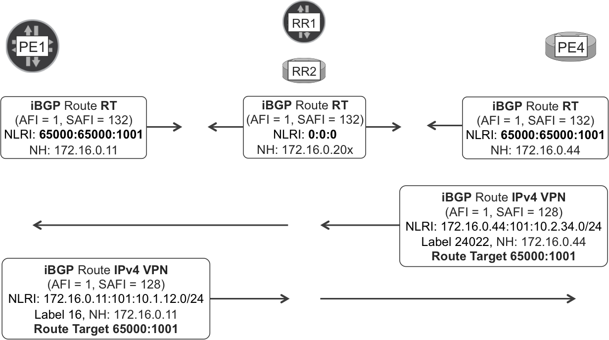
Figure 3-6. Route Target Constraint
This mechanism ensures that PEs only receive the VPN routes that they are interested in: nothing more, nothing less. Also, every time a VRF is added, removed, or modified at PE1, its RT routes are updated accordingly, potentially triggering tailored VPN route updates from the RRs. There is no need for a full route refresh anymore. And the same reasoning applies to PE2, too.
Note that the term VPN (and not L3VPN) has been used intentionally. RT routes are not bound to any particular type of VPN NLRI. Indeed, RTC is a conceptually universal mechanism. In Junos, every VPN NLRI supports RTC. In IOS XR, as of this writing, IPv4 and IPv6 Unicast VPN (SAFI=128) NLRIs support RTC.
RTC—RR Configuration
Following is the Junos RR additional configuration:
Example 3-41. RTC configuration at RR1 (Junos)
protocols {
    bgp {
        group CLIENTS {
            family route-target advertise-default;
}}}
Here is the equivalent for IOS XR PE:
Example 3-42. RTC configuration at RR2 (IOS XR)
router bgp 65000
 address-family ipv4 rt-filter
 !
 neighbor-group CLIENTS
  address-family ipv4 rt-filter
   default-originate
!
The ipv4 notation is due to the fact that RT NLRI has AFI=1. But RT prefixes also determine the distribution of non-IPv4 VPN routes such as IPv6 Unicast VPN.
Remember that RT prefixes are not reflected. Also, there is no need to negotiate the RT NLRI on the inter-RR iBGP sessions.
RTC—PE Configuration
The following example provides the Junos PE additional configuration:
Example 3-43. RTC configuration at PE1 (Junos)
1     protocols {
2         bgp group iBGP-RR family route-target;
3     }
4     routing-options {
5         rib inet.3 {
6             static {
7                 route 172.16.0.201/32 discard;
8                 route 172.16.0.202/32 discard;
9     }}}
RRs advertise an RT default prefix whose BGP next hop equals the RR’s local loopback (172.16.0.201 or 172.16.0.202). In this example, the RRs do not run any MPLS protocols, so their loopbacks are missing from the PE1’s inet.3 routing table. Without the static routes in lines 4 through 8, the RT prefixes would be hidden at PE1—effectively disrupting the L3VPN service.
Alternatively, you can configure: set routing-options resolution rib bgp.rtarget.0 resolution-ribs [ inet.3 inet.0 ].
Finally, Example 3-44 shows here is the additional configuration at an IOS XR PE.
Example 3-44. RTC configuration at PE2 (IOS XR)
router bgp 65000
 address-family ipv4 rt-filter
 !
 neighbor-group RR
  address-family ipv4 rt-filter
!
Note
The RT static route concept is explored in Chapter 9.
Coupling MPLS Services to Transport Planes
Every MPLS service has its own requirements. Let’s suppose that you want to do the following:
-
Transport high-volume Internet traffic through a set (#1) of core RSVP-TE LSPs that take the available bandwidth and the actual link utilization into account. In this way (fully covered in Chapter 14) you can minimize packet loss by avoiding situations in which some links are underutilized, whereas others are saturated.
-
Transport low-volume VPN traffic by following the IGP. This traffic does not contribute to link bandwidth significantly, and the shortest path is preferred. For this service, LDP or node-SID SPRING are perfectly fine transport alternatives.
-
Transport the traffic from critical VPNs—or specific flows within these VPNs—with a new set (#2) of RSVP-TE LSPs that have fast restoration paths; and you don’t want the Internet traffic to use these LSPs.
The solution is to define three loopback addresses on every LSR and LER:
-
Loopback address A is reachable through RSVP-TE LSPs named with suffix PLANE_A. Internet BGP routes have their iBGP next hop set to this address.
-
Loopback address B is advertised as a FEC in LDP. Most VPN routes have their iBGP next hop set to this address.
-
Loopback address C is reachable through RSVP-TE LSPs named with suffix PLANE_C. Certain VPN routes have their iBGP next hop set to this address.
Let’s see how to configure several global loopback addresses, how to bind them to RSVP-TE LSPs or LDP FECs, and how to change the iBGP next hop.
Configuring Several Loopbacks in the Default Instance
Junos supports a maximum of one loopback IFL per instance. You can configure several IPv4 addresses on the same unit as follows:
Example 3-45. Multiple global loopback address—PE1 (Junos)
interfaces {
    lo0 {
        family inet {
            address 172.16.0.11/32 primary;
            address 172.16.1.11/32;
            address 172.16.2.11/32;
}}}
These are loopback addresses A, B, and C mentioned previously. The router ID is better set explicitly to the primary loopback address A.
IOS XR provides two options: either configuring several loopback interfaces, or configuring several addresses on the same interface. Let’s look at the first option:
Example 3-46. Multiple global loopback address—PE4 (Junos)
interface Loopback0
 ipv4 address 172.16.0.44 255.255.255.255
 ipv4 address 172.16.1.44 255.255.255.255 secondary
 ipv4 address 172.16.2.44 255.255.255.255 secondary
!
Signaling LSPs to Different Loopback Addresses
Let’s carry on with the example, this time focusing on the signaling and forwarding between PE1 and PE4. From PE1’s perspective, the remote PE is PE4, and vice versa.
Plane A—RSVP-TE LSPs to the remote PE’s router ID
These are the two RSVP-TE LSPs signaled on plane A: PE1→PE4_PLANE-A and PE4→PE1_PLANE-A. They have as a destination the remote PE’s loopback address A.
By default, Junos only installs a route to the RSVP-TE LSP destination (to address) in the inet.3 routing table. This is exactly what we want in this case.
Example 3-47. RSVP-TE LSP plane A, rooted at PE1 (Junos)
protocols {
    mpls {
        label-switched-path PE1--->PE4_PLANE-A {
            to 172.16.0.44;
}}}
As for IOS XR, by default there is no prefix bound to a RSVP-TE LSP. Indeed, autoroute is not turned on by default; you must configure it explicitly.
Now, the autoroute announce feature automatically uses the RSVP-TE LSPs as a next hop for all the destinations that are at or behind the tail end. So, PE4’s CEF sees the three PE1’s loopback IP addresses as reachable via the PE4→PE1_PLANE_A LSP. This is not what you want in this scenario, and the solution is not to use autoroute announce. There are several alternative methods for coupling prefixes to a LSP. One option is to use static routes, but it is much better to use a dynamic method that takes the IGP metric into account: this is the autoroute destination feature.
Example 3-48. RSVP-TE LSP plane A, rooted at PE4 (IOS XR)
1     interface tunnel-te1101
2      ipv4 unnumbered Loopback 0
3      signalled-name PE4--->PE1_PLANE-A
4      autoroute destination 172.16.0.11
5      !
6      destination 172.16.0.11
7      record-route
8      path-option 1 dynamic
9     !
It is line 4, not line 6, that determines what is installed at PE4’s CEF. In this case, PE4 sees only one prefix as reachable via PE4→PE1_PLANE_A: 172.16.0.11.
Note
The IOS XR autoroute announce feature is equivalent to Junos’ shortcuts, which are briefly described in Chapter 16.
Plane B—controlling LDP label bindings
The two vendors covered by this book have a different default behavior:
-
Junos PE1 only advertises a label mapping for one local FEC: its primary loopback address (A). As for remote FECs, it uses the ordered label distribution control mode, which means that it only advertises label mappings for those remote FECs for which it has already received label mappings from the downstream LSR.
-
IOS XR advertises a label mapping for all the local and remote (IGP) FECs in independent mode. This means that PE2, P2, and PE4 advertise a label mapping for all the loopback addresses (A, B, and C) of all the PEs, including PE1 and PE4.
Is the default implementation a valid one in this scenario? Let’s focus on plane A first.
In both Junos and IOS XR, if a remote FEC is reachable via a RSVP-TE LSP and via LDP label mappings, RSVP-TE is preferred. So RSVP-TE LSPs PE1→PE4_PLANE_A and PE4→PE1_PLANE_A take precedence over LDP. Only if the RSVP-TE LSPs cannot be signaled, for whatever reason, does LDP act as a fallback mechanism.
But this might not be your preferred option. Suppose that all the LSRs in the network are capable of IP routing Internet packets in the global instance. Although this scenario deviates from the first classical MPLS use case, it is a common practice in international carriers because it provides hop-by-hop control. In this case, you might prefer the fallback mechanism in plane A—dedicated in this example to the Internet service—not to be LDP, but hop-by-hop classical (unlabeled) IP routing. In this case, it is necessary to filter loopback address A out of LDP advertisements.
As for plane B, Junos P1 only advertises a label mapping for PE1’s loopback address B if it has previously received the corresponding label mapping from PE1.
Finally, let’s assume that LDP is a desirable fallback mechanism for plane C. Putting this all together, LDP must advertise label mappings for planes B and C, but not for plane A.
Following is the required configuration at Junos PE1:
Example 3-49. Controlling LDP label bindings for Local FECs—PE1 (Junos)
1     protocols {
2         ldp egress-policy PL-LDP-EGRESS;
3     }
4     policy-options {
5         policy-statement PL-LDP-EGRESS {
6             term LOOPBACK-B-C {
7                 from {
8                     route-filter 172.16.1.11/32;
9                     route-filter 172.16.2.11/32;
10                }
11                then accept;
12            }
13            term REST {
14                then reject;
15    }}}
Junos PE3 needs a similar configuration—just by adapting lines 8 and 9 to its local addressing—and P1 does not require any additional changes.
The required configuration on all the IOS XR core routers (PE2, P2, and PE4) is shown in Example 3-50.
Example 3-50. Controlling LDP label bindings—IOS XR
mpls ldp
 address-family ipv4
  label
   local
    allocate for ALL-LOCAL-PLANE-B-C
!
ipv4 access-list AL-LOCAL-PLANE-B-C
 10 permit ipv4 172.16.1.0 0.0.0.255 any
 20 permit ipv4 172.16.2.0 0.0.0.255 any
 30 deny ipv4 any any
!
Plane C—RSVP-TE LSPs to a secondary loopback address
These are the two RSVP-TE LSPs signaled on plane C: PE1→PE4_PLANE-C and PE4→PE1_PLANE-C. They are coupled to the remote PE’s loopback address C.
Note
In both Junos and IOS XR, by default a RSVP-TE LSP must be targeted to the tail end’s router ID. In this scenario, this is loopback address A. You can relax this requirement in Junos with the inter-domain knob.
Taking into account this boundary condition, here is the configuration at PE1:
Example 3-51. RSVP-TE LSP plane C, rooted at PE1 (Junos)
1     protocols {
2         mpls {
3             label-switched-path PE1--->PE4_PLANE-C {
4                 to 172.16.0.44;
5                 no-install-to-address;
6                 install 172.16.2.44;
7     }}}
With the previous configuration, the LSP is a next hop for the 172.16.2.44/32 route (line 6) at PE1’s inet.3 table. But it is not a next hop for 172.16.0.44/32 (line 5).
Here is the IOS XR configuration at PE4.
Example 3-52. RSVP-TE LSP plane C, rooted at PE4 (IOS XR)
1     interface tunnel-te1103
2      ipv4 unnumbered Loopback 0
3      signalled-name PE4--->PE1_PLANE-C
4      autoroute destination 172.16.2.11
5      !
6      destination 172.16.0.11
7      record-route
8      path-option 1 dynamic
9     !
It is line 4, not line 6, that determines what is installed at PE4’s CEF. In this case, PE4 sees only one prefix as reachable via PE4→PE1_PLANE_C: 172.16.2.11.
There is an interesting implementation difference between Junos install and IOS XR autoroute destination. Junos calculates the 172.16.2.44/32 FEC metric as the shortest IGP path to the LSP’s tail end (172.16.0.44). IOS XR, on the other hand, calculates it as the shortest IGP path to the FEC itself (172.16.2.11, not 172.16.0.11).
In this example, there is no difference because the FEC is local to the LSP’s tail end. But there are other use cases of this technique—mainly Traffic Engineering—for which the LSP’s tail end may be en route to the FEC; however, the FEC is still one or more hops beyond. In this case, the previous implementation difference is relevant. There is a way to make Junos use the FEC metric—based on LDP tunneling and LDP policies—but it is beyond the scope of this book.
Changing the Service Routes’ BGP Next Hop
Now that there are three transport planes, let’s couple the services to them according to the previously stated requirements. No change is required on plane A, because the BGP next-hop self (NHS) action automatically picks the primary loopback address (A).
Let’s see plane B in Junos:
-
If PE1 advertises IP VPN prefixes directly from the VRF (this topic was further discussed earlier in this chapter), the way to go is making the VRF export policy execute a
then next-hop 172.16.1.11action. -
If PE1 advertises IP VPN prefixes from the main IP VPN table, the
then next-hop 172.16.1.11action must be applied at the iBGP-RR group export policy, where you can also match the RTs in order to achieve a good granularity. Don’t forget in this case to configurevpn-apply-exportunder the group, too.
Example 3-53 shows the procedure in IOS XR.
Example 3-53. Changing BGP next hop for L3VPN routes—PE4 (IOS XR)
1     router bgp 65000
2      neighbor-group RR
3       address-family vpnv4 unicast
4        route-policy PL-VRF-NH-CHANGE out
5       !
6       address-family vpnv6 unicast
7        route-policy PL-VRF-A-NH-CHANGE out
8     !
9     route-policy PL-VRF-NH-CHANGE
10      if extcommunity rt matches-any RT-VPN-A then
11        set next-hop 172.16.1.44
12      endif
13      pass
14    end-policy
15    !
16    extcommunity-set rt RT-VPN-A
17      65000:1001
18    end-set
19    !
For IPv6 Unicast VPN prefixes (line 6), the next hop changes to ::ffff:172.16.1.44 even if it’s configured to be 172.16.1.44. Good!
The approach for plane C is identical, except that further per-prefix granularity may be configured in the policies.