Now, we arrive at the fun part—the neural network. The complete code to train this model is available at the following link: https://github.com/mlwithtf/mlwithtf/blob/master/chapter_02/training.py

To train the model, we'll import several more modules:

 import sys, os
 import tensorflow as tf
 import numpy as np
 sys.path.append(os.path.realpath('..'))
 import data_utils
 import logmanager 

Then, we will define a few parameters for the training process:

 batch_size = 128
 num_steps = 10000
 learning_rate = 0.3
 data_showing_step = 500

After that, we will use the data_utils package to load the dataset that was downloaded in the previous section:

 dataset, image_size, num_of_classes, num_of_channels =  
 data_utils.prepare_not_mnist_dataset(root_dir="..")
 dataset = data_utils.reformat(dataset, image_size, num_of_channels,   
 num_of_classes)
 print('Training set', dataset.train_dataset.shape,  
 dataset.train_labels.shape)
 print('Validation set', dataset.valid_dataset.shape,  
 dataset.valid_labels.shape)
 print('Test set', dataset.test_dataset.shape,  
 dataset.test_labels.shape)

We'll start off with a fully-connected network. For now, just trust the network setup (we'll jump into the theory of setup a bit later). We will represent the neural network as a graph, called graph in the following code:

 graph = tf.Graph()
 with graph.as_default():
 # Input data. For the training data, we use a placeholder that will  
 be fed
 # at run time with a training minibatch.
 tf_train_dataset = tf.placeholder(tf.float32,
 shape=(batch_size, image_size * image_size * num_of_channels))
 tf_train_labels = tf.placeholder(tf.float32, shape=(batch_size,  
 num_of_classes))
 tf_valid_dataset = tf.constant(dataset.valid_dataset)
 tf_test_dataset = tf.constant(dataset.test_dataset)
 # Variables.
 weights = {
 'fc1': tf.Variable(tf.truncated_normal([image_size * image_size *  
 num_of_channels, num_of_classes])),
 'fc2': tf.Variable(tf.truncated_normal([num_of_classes,  
 num_of_classes]))
 }
 biases = {
 'fc1': tf.Variable(tf.zeros([num_of_classes])),
 'fc2': tf.Variable(tf.zeros([num_of_classes]))
 }
 # Training computation.
 logits = nn_model(tf_train_dataset, weights, biases)
 loss = tf.reduce_mean(
 tf.nn.softmax_cross_entropy_with_logits(logits=logits,  
 labels=tf_train_labels))
 # Optimizer.
 optimizer =  
 tf.train.GradientDescentOptimizer(learning_rate).minimize(loss)
 # Predictions for the training, validation, and test data.
 train_prediction = tf.nn.softmax(logits)
 valid_prediction = tf.nn.softmax(nn_model(tf_valid_dataset,  
 weights, biases))
 test_prediction = tf.nn.softmax(nn_model(tf_test_dataset, weights,  
 biases))
 The most important line here is the nn_model where the neural  
 network is defined:
 def nn_model(data, weights, biases):
 layer_fc1 = tf.matmul(data, weights['fc1']) + biases['fc1']
 relu_layer = tf.nn.relu(layer_fc1)
 return tf.matmul(relu_layer, weights['fc2']) + biases['fc2']

The loss function that is used to train the model is also an important factor in this process:

 loss = tf.reduce_mean(
 tf.nn.softmax_cross_entropy_with_logits(logits=logits,  
 labels=tf_train_labels))
 # Optimizer.
 optimizer =  
 tf.train.GradientDescentOptimizer(learning_rate).minimize(loss)

This is the optimizer being used (Stochastic Gradient Descent) along with the learning_rate (0.3) and the function we're trying to minimize (softmax with cross-entropy).

The real action, and the most time-consuming part, lies in the next and final segment—the training loop:

We can run this training process using the following command in the chapter_02 directory:

python training.py

Running the procedure produces the following output:

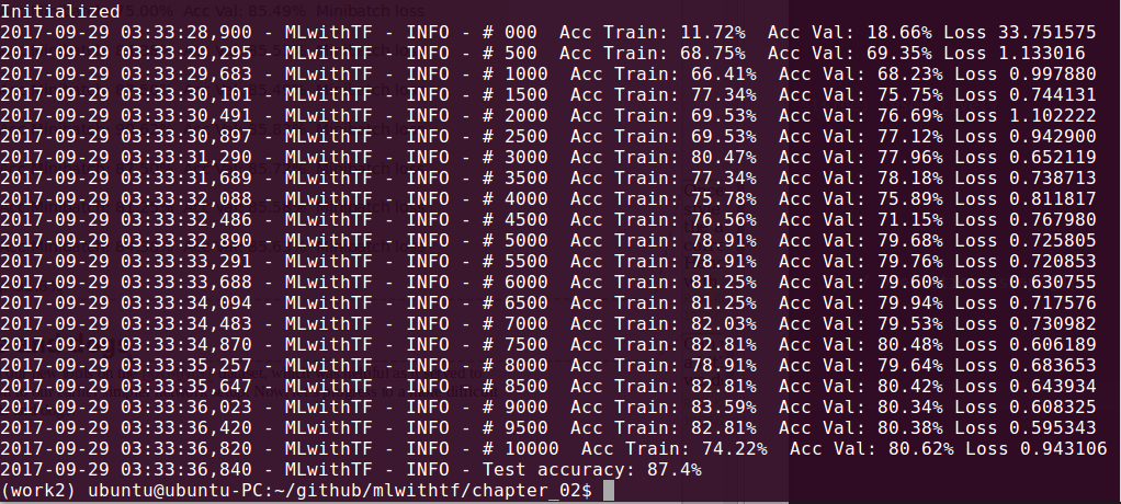
We are running through hundreds of cycles and printing indicative results once every 500 cycles. Of course, you are welcome to modify any of these settings. The important part is to appreciate the cycle:

• We will cycle through the process many times.
• Each time, we will create a mini batch of photos, which is a carve-out of the full image set.
• Each step runs the TensorFlow session and produces a loss and a set of predictions. Each step additionally makes a prediction on the validation set.
• At the end of the iterative cycle, we will make a final prediction on our test set, which is a secret up until now.
• For each prediction made, we will observe our progress in the form of prediction accuracy.

We did not discuss the accuracy method earlier. This method simply compares the predicted labels against known labels to calculate a percentage score:

 def accuracy(predictions, labels): 
  return (100.0 * np.sum(np.argmax(predictions, 1) == 
   np.argmax(labels, 1)) 
          / predictions.shape[0])

Just running the preceding classifier will yield accuracy in the general range of 85%. This is remarkable because we have just begun! There are much more tweaks that we can continue to make.