CNNs are more advanced neural networks specialized for machine learning with images. Unlike the hidden layers we used before, CNNs have some layers that are not fully connected. These convolutional layers have depth in addition to just width and height. The general principle is that an image is analyzed patch by patch. We can visualize the 7x7 patch in the image as follows:

This reflects a 32x32 greyscale image, with a 7x7 patch. Example of sliding the patch from left to right is given as follows:

If this were a color image, we'd be sliding our patch simultaneously over three identical layers.

You probably noticed that we slid the patch over by one pixel. That is a configuration as well; we could have slid more, perhaps by two or even three pixels each time. This is the stride configuration. As you can guess, the larger the stride, the fewer the patches we will end up covering and thus, the smaller the output layer.

Matrix math, which we will not get into here, is performed to reduce the patch (with the full depth driven by the number of channels) into an output depth column. The output is just a single in height and width but many pixels deep. As we will slide the patch across, over, and across iteratively, the sequence of depth columns form a block with a new length, width, and height.

There is another configuration at play here—the padding along the sides of the image. As you can imagine, the more padding you have the more room the patch has to slide and veer off the edge of the image. This allows more strides and thus, a larger length and width for the output volume. You'll see this in the code later as padding='SAME' or padding='VALID'.

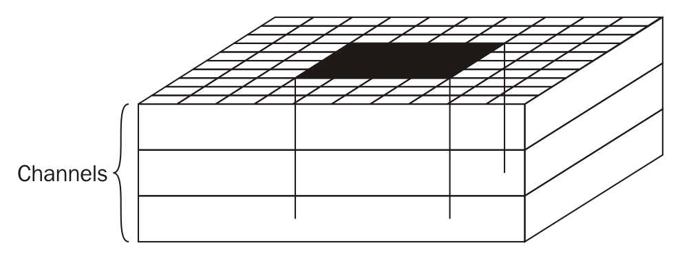
Let's see how these add up. We will first select a patch:

However, the patch is not just the square, but the full depth (for color images):

We will then convolve that into a 1x1 volume, but with depth, as shown in the following diagram. The depth of the resulting volume is configurable and we will use inct_depth for this configuration in our program:

Finally, as we slide the patch across, over, and across again, through the original image, we will produce many such 1x1xN volumes, which itself creates a volume:

We will then convolve that into a 1x1 volume.

Finally, we will squeeze each layer of the resulting volume using a POOL operation. There are many types, but simple max pooling is typical:

Much like with the sliding patches we used earlier, there will be a patch (except this time, we will take the maximum number of the patch) and a stride (this time, we'll want a larger stride to squeeze the image). We are essentially reducing the size. Here, we will use a 3x3 patch with a stride of 2.