IV.3

Historical Simulation

IV.3.1 INTRODUCTION

Historical simulation as a method for estimating VaR was introduced in a series of papers by Boudoukh et al. (1998) and Barone-Adesi et al. (1998, 1999). A recent survey suggests that about three-quarters of banks prefer to use historical simulation rather the parametric linear or Monte Carlo VaR methodologies.¹ Why should this be so – what are the advantages of historical simulation over the other two approaches?

The main advantage is that historical VaR does not have to make an assumption about the parametric form of the distribution of the risk factor returns. Although the other models can include skewed and heavy tailed risk factor returns, they must still fit a parametric form for modelling the multivariate risk factor returns. And usually the dependencies between risk factors in this multivariate distribution are assumed to be much simpler than they are in reality.

For instance, the parametric linear model assumes that risk factor return dependencies are linear and are fully captured by one or more correlation matrices. This is also commonly assumed in Monte Carlo VaR, although here it is possible to assume more complex dependency structures as explained in the next chapter. Also, the parametric linear VaR model is a one-step model, based on the assumption that risk factor returns are i.i.d. There is no simple way that path-dependent behaviour such as volatility clustering can be accounted for in this framework. Monte Carlo VaR models can easily be adapted to include path dependency, as we shall see in the next chapter. But still, they have to assume some idealized form for the risk factor evolution. For instance, Monte Carlo VaR may assume that volatility and correlation clustering are captured by a GARCH model.

Historical VaR does not need to make any such parametric assumption, and instead the dynamic evolution and the dependencies of the risk factors are inferred directly from historical observations. This allows the model to assess the risk of complex path-dependent products or the risk of simple products, but still include the dynamic behaviour of risk factors in a natural and realistic manner.

Historical VaR is also not limited to linear portfolios, as the parametric linear VaR model is. So the advantages of historical simulation over the parametric linear model are very clear. However, both historical and Monte Carlo VaR may be applied to any type of portfolio. So, what are the advantages, if any, of the historical VAR model over Monte Carlo VaR? In fact, let us rephrase this question: ‘Which model has the most substantial limitations?’ The Monte Carlo VaR model suffers from the drawback of being highly dependent on finding a suitably realistic risk factor returns model. Likewise, in the course of this chapter and Chapter IV.5 we shall show that if the historical VaR model is to be used then several challenges must be addressed.²

Firstly, it is difficult to apply historical VaR to risk assessments with a horizon longer than a few days. This is because data limitations are a major concern. To avoid unstable VaR estimates when the model is re-estimated day after day, we require a considerable amount of historical data. Even 4 years of daily historical data are insufficient for an acceptable degree of accuracy unless we augment the historical model in some way.³ Overlapping data on h-day returns could be used, but we shall show in Section IV.3.2.7 that this can seriously distort the tail behaviour of the portfolio return distribution.

Hence, almost always, we base historical VaR estimation on the distribution of daily portfolio returns (or P&L) and then scale the 1-day VaR estimate to an h-day horizon. But finding an appropriate scaling rule for historical VaR is not easy, as we shall see in Section IV.3.2. Also, scaling up the VaR for option portfolios in this way assumes the portfolio is rebalanced daily over the risk horizon to return risk factor sensitivities to their value at the time the VaR is measured. That is, we can measure what I call the dynamic VaR of an option portfolio, but we shall see in Section IV.5.4 that the standard historical model is very difficult to apply to static VaR estimation, i.e. the VaR estimate based on no trading over the risk horizon.

We should recall that a vital assumption in all VaR models is that the portfolio remains the same over the risk horizon, in a sense that will be made more precise in Section IV.5.2.4. Since the historical simulation model forecasts future returns using a large sample of historical data, we have to recreate a historical ‘current’ returns series by holding the portfolio characteristics constant. For instance, in cash equity portfolios the current portfolio weights on each stock and the current stock betas are all held constant as we simulate ‘current’ portfolio returns for the entire historical data period. Hence, an implicit assumption of historical VaR is that the current portfolio, which is optimal now, would also have been the portfolio of choice during every day of the historical sample.⁴ Thus a criticism of historical VaR that cannot always be levelled at the other two approaches is that it is unrealistic to assume that we would have held the current portfolio when market conditions were different from those prevalent today.

A difficulty that needs addressing when implementing the historical VaR model is that a long data history will typically encompass several regimes in which the market risk factors have different behaviour. For instance, during a market crash the equity risk factor volatilities and correlations are usually much higher than they are during a stable market. If all the historical data are treated equally, the VaR estimate will not reflect the market conditions that are currently prevailing. In Section IV.3.3 we shall recommend a parametric volatility adjustment to the data, to account for volatility clustering regimes in the framework of historical simulation.

Given the substantial limitations, it is difficult to understand why so many banks favour historical VaR over Monte Carlo VaR models. Maybe market risk analysts rely very heavily on historical data, because (usually) it is available, and they draw some confidence from a belief that if a scenario has occurred in the past, it will reoccur within the risk horizon of the model. But in my view their reliance on historical data is misplaced. Too often, when a crisis occurs, it is a scenario that has not been experienced in the past.

In my view, the great advantage of Monte Carlo simulation is that is uses historical data more intelligently than standard historical simulation does. After fitting a parametric behavioural model (preferably with volatility clustering and non-normal conditional return distributions) to historical data, the analyst can simulate many thousands of possible scenarios that could occur with that model. They do not assume that the one, experienced scenario that led to that model will also be the one, of all the consistent scenarios, that is actually realized over the risk horizon. A distinct advantage of the filtered historical simulation approach (which is described in Section IV.3.3.4. over standard historical simulation is that it combines Monte Carlo simulation based on volatility clustering with the empirical non-normal return distributions that have occurred in the past.

The aim of the present chapter is to explain how to use historical VaR to obtain realistic VaR estimates. We focus on linear portfolios here, leaving the more complex (and thorny) problem of the application of historical VaR to option portfolios to Chapter IV.5. We shall propose the following, very general steps for the implementation of historical VaR for linear portfolios:

• Obtain a sufficiently long period of historical data.
• Adjust the simulated portfolio returns to reflect the current market conditions.
• Fit the empirical distribution of adjusted returns.
• Derive the VaR for the relevant significance level and risk horizon.

We now detail the structure of this chapter.

Section IV.3.2 focuses on the properties of standard historical VaR, focusing on the problems we encounter when scaling VaR from a 1-day to an h-day horizon. We describe how the stable distribution assumption provides a method for estimating a scale exponent and we explain how risk factor scale exponents can relate to a power law scaling of VaR for linear portfolios. Then we estimate this exponent for major equity, foreign exchange and interest rate risk factors. The case for non-linear portfolios is more difficult, because portfolio returns need not be stable even when the risk factor returns are stable; also, even if it was considered appropriate to scale equity, commodity, interest rate, and exchange rate risk factors with the square root of time, this is definitely not appropriate for scaling volatility.

Section IV.3.3 concerns the preparation of the historical data set. It is motivated by a case study which demonstrates that when VaR is estimated using equal weighing of historical returns it is the choice of data, rather than the modelling approach, that really determines the accuracy of a VaR estimate. We emphasize the need to adjust historical data so that they more accurately reflect current market conditions, and for short-term VaR estimation we recommend a volatility adjustment of historical returns. The section ends with a description and an illustration of filtered historical simulation, and a discussion of its advantages over standard historical simulation.

Section IV.3.4 provides advice on estimating historical VaR at extreme quantiles when only a few years of daily data are available. Non-parametric smoothing and parametric fitting of the empirical distribution of (adjusted) portfolio returns can improve the precision of historical VaR at the 99% and higher confidence levels. Non-parametric methods include the Epanechnikov kernel and the Gaussian kernel, and we also discuss several parametric methods including the Johnson SU distribution, the Cornish–Fisher expansion, and the generalized Pareto and other extreme value distributions.

Up to this point we will have considered the measurement of VaR at the portfolio level. Now we consider the historical systematic VaR, which is based on the risk factor mapping of different linear portfolios. Section IV.3.5 describes the estimation of historical VaR when portfolio returns are a linear function of either asset or risk factor returns. Several case studies and examples of historical VaR modelling for cash flow, equity and commodity portfolios are presented, and we describe how systematic historical VaR may be disaggregated into stand-alone VaR and marginal VaR components.

Section IV.3.6 shows how to estimate the conditional VaR or expected tail loss in a historical VaR model. We give analytic formulae for computing ETL when the historical returns are fitted with a parametric form, and conclude with an example. The results confirm that fitting a Johnson distribution to the moments of the empirical returns can be a useful technique for estimating ETL (and VaR) at high levels of confidence. Section IV.3.7 summarizes and concludes.

IV.3.2 PROPERTIES OF HISTORICAL VALUE AT RISK

This section provides a formal definition of historical VaR and summarizes the approach for different types of portfolios. We then consider the constraints that this framework places on the historical data and justify our reasons for basing historical VaR estimation on daily returns. This leads to a discussion on a simple scaling rule for extending a 1-day historical VaR to a historical VaR at longer risk horizons.

IV.3.2.1 Definition of Historical VaR

The 100α% h-day historical VaR, in value terms, is the α quantile of an empirical h-day discounted P&L distribution. Or, when VaR is expressed as a percentage of the portfolio's value, the 100α% h-day historical VaR is the α quantile of an empirical h-day discounted return distribution. The percentage VaR can be converted to VaR in value terms: we just multiply it by the current portfolio value.

Historical VaR may be applied to both linear and non-linear portfolios. When a long-only (or short-only) linear portfolio is not mapped to risk factors, a historical series of returns on the portfolio is constructed by holding the current portfolio weights constant and applying these to the asset returns to reconstruct a constant weighted portfolio returns series. An example is given in Section IV.3.4.2.

But the concept of a ‘return’ does not apply to long-short portfolios, because they could have a value of zero (see Section I.1.4.4). So in this case we generate the portfolio's P&L distribution directly, by keeping the current portfolio holdings constant, and calculate the VaR in nominal terms at the outset. This approach is put into practice in the case study of Section IV.3.5.6.

When a portfolio is mapped to risk factors, the risk factor sensitivities are assumed constant at their current values and are applied to the historical risk factor returns to generate the portfolio return distribution. Case studies to illustrate this approach are provided in Sections IV.3.4.1 and IV.3.6.3.

IV.3.2.2 Sample Size and Data Frequency

For assessing the regulatory market risk capital requirement, the Basel Committee recommends that a period of between 3 and 5 years of daily data be used in the historical simulation model. But the sample size and the data frequency are not prescribed by any VaR model: essentially these are matters of subjective choice.

Sample Size

If VaR estimates are to reflect only the current market conditions rather than an average over a very long historical period, it seems natural to use only the most recent data. For instance, if markets have behaved unusually during the past year, we may consider using only data from the last 12 months. A relatively short data period may indeed be suitable for the linear and Monte Carlo VaR models. The covariance matrix will then represent only recent market circumstances. But the historical simulation VaR model requires much more than just estimating the parameters of a parametric return distribution. It requires one to actually build the distribution from historical data, and then to focus on the tail of this distribution. So, with historical simulation, the sample size has a considerable influence on the precision of the estimate.

Since VaR estimates at the 99% and higher confidence levels are the norm, it is important to use a large number of historical returns.⁵ For a 1% VaR estimation, at least 2000 daily observations on all the assets or risk factors in the portfolio should be used, corresponding to at least 20 data points in the 1% tail. But even 2000 observations would not allow the 0.1% VaR to be estimated with acceptable accuracy. See Section IV.3.4 for a discussion on improving the precision of historical VaR at very high confidence levels.

However, there are several practical problems with using a very large sample. First, collection of a data on all the instruments in the portfolio can be a formidable challenge. Suppose the portfolio contains an asset that has only existed for one year: how does one obtain more than one year of historical prices? Second, in the historical model the portfolio weights, or the risk factor sensitivities if the model has a risk factor mapping, are assumed constant over the entire historical data period. The longer the sample period the more questionable this assumption becomes, because a long historical period is likely to cover several different market regimes in which the market behaviour would be very different from today.

Data Frequency

The choice of sample size is linked to the choice of data frequency. It is easier to obtain a large sample of high frequency data than of low frequency data. For instance, to obtain 500 observations on the empirical distribution we would require a 20-year sample if we used 10-day returns, a 10-year sample if we used weekly returns, a 2-year sample if we used daily returns, and a sample covering only the last month or so if we used hourly returns.

For computing VaR-based trading limits it would be ideal if the data warehouse captured intra-day prices on all the risk factors for all portfolios, but in most financial institutions today this is computationally impractical. Since it is not appropriate to hold the current portfolio weights and sensitivities constant over the past 10 years or more, and since also the use of such a long historical period is hardly likely to reflect the current circumstances, it is not appropriate to base historical VaR models on weekly or monthly data. There are also insufficient data to measure historical VaR at extreme quantiles using an empirical distribution based on weekly or monthly returns.

Hence, the historical h-day VaR is either scaled up from a 1-day VaR estimate based on historical data on the portfolio's daily returns or P&L, or we might consider using multi-step simulation. In the next subsection we consider the first of these solutions, leaving our discussion of multi-step simulation to Sections IV.3.2.7 and IV.3.3.4.

IV.3.2.3 Power Law Scale Exponents

In this subsection we discuss how to estimate the 100α% h-day historical VaR as some power of h times the 100α% 1-day historical VaR, assuming the 100α% 1-day historical VaR has been computed (as the α quantile of the daily returns or P&L distribution).

In Section IV.1.5.4 we showed that the assumption that returns are normal and i.i.d. led to a square-root-of-time rule for linear VaR estimates. For instance, to estimate the 10-day VaR we take the square root of 10 times the 1-day VaR. The square-root-of-time rule applies to linear VaR because it obeys the same rules as standard deviation, either approximately over short risk horizons or over all horizons when the expected return is equal to the discount rate. But in the historical model the VaR corresponds to a quantile of some unspecified empirical distribution and quantiles do not obey a square-root-of-time rule, except when the returns are i.i.d. and normally distributed.

Scaling rules for quantiles can only be derived by making certain assumptions about the distribution. Suppose we have an i.i.d. process for a random variable X, but that X is not necessarily normally distributed. Instead we just assume that X has a stable distribution.⁶ When a distribution is ξ-stable then the whole distribution, including the quantiles, scales as h^1/ξ. For instance, in a normal distribution ξ = 2 and we say that its scale exponent is . More generally, the scale exponent of a stable distribution is ξ⁻¹. This exponent is used to scale the whole distribution of returns, not just its standard deviation, and in VaR applications we use it to scale the quantiles of the distribution.

Let x_{h, α} denote the α quantile of the h-day discounted log returns. We seek ξ such that

In other words, taking logs of the above,

Hence ξ can be estimated as the slope of graph with ln (x_{h, α}) − ln (x_{1, α}) on the horizontal axis and ln (h) on the vertical axis. If the distribution is stable the graph will be a straight line and ξ will not depend on the choice of α. Nor should it vary much when different samples are used, provided the sample contains sufficient data to estimate the quantiles accurately. When a constant scale exponent corresponding to (IV.3.1) exists, we say that the log return obeys a power law scaling rule with exponent ξ⁻¹.

IV.3.2.4 Case Study: Scale Exponents for Major Risk Factors

In this section we illustrate the estimation of (IV.3.2) for some major risk factors, and use the estimates for different values of α to investigate whether their log returns are stable. First we estimate the scale exponent using (IV.3.2), as a function of α, for the S&P 500 index. We base our results on daily data over a very long period from 3 January 1950 until 10 March 2007 and then ask how sensitive the estimated scale exponent is to (a) the choice of quantile α, and (b) the sample data.

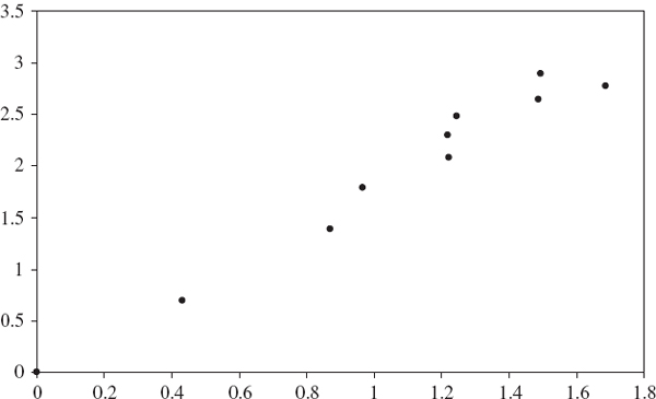
The spreadsheet for Figure IV.3.1 aggregates daily log returns into h-day log returns for values of h from 2 to 20, and for a fixed α computes the quantile of the h-day log returns, x_{h, α}. First ξ is estimated as the slope of the log-log plot of the holding period versus the quantile ratio, as explained above. Figure IV.3.1 illustrates the graph for α = 5% where the quantiles are based on the entire sample period. The scale exponent ξ⁻¹ is the reciprocal of the slope of the best fit line, which in Figure IV.3.1 is 0.50011. This indicates that a square-root scaling rule for 5% quantiles of the S&P 500 index is indeed appropriate.

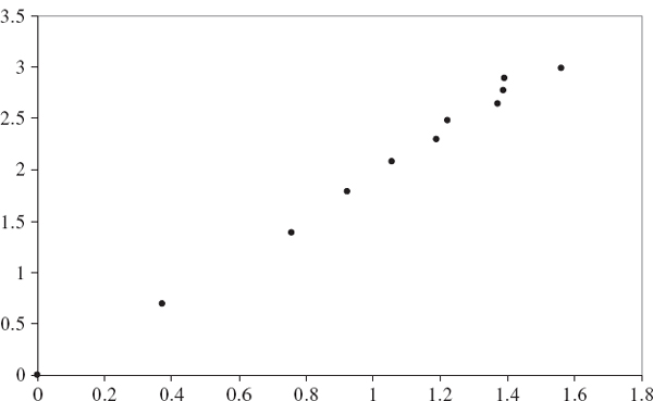
Figure IV.3.1 Log-log plot of holding period versus 5% quantile ratio: S&P 500 index

Table IV.3.1 Estimated values of scale exponent for S&P 500 index

However, there is some variation when different quantiles and different sample periods are chosen. Table IV.3.1 records the reciprocal of the slope of the log-log plot for different values of α and when the quantiles are based on three different sample periods: from the beginning of January 1950, 1970 and 1990 onward. Using data from 1990 onward the scale exponent for the 10% and 0.1% quantiles is less than 0.5, although it should be noted that with little more than 4000 data points, the 0.1% quantile may be measured imprecisely. Still, based on data since 1990 only, it appears that the scale exponent for the 1% quantile of the S&P 500 index is closer to 0.45 than to 0.5.

We also estimate the scale exponent for three other important risk factors, the $/£ exchange rate and two US Treasury interest rates at 3 months and 10 years, using daily data since January 1971. The relevant log-log plots are shown in Figures IV.3.2–IV.3.4, each time based on α = 5% and the results for other quantiles are shown in Table IV.3.2.⁷ The $/£ exchange rate has a lower estimated scale exponent than the interest rates and, again except for the 0.1% and 10% quantiles, appears to be close to 0.5. So, like the S&P 500 index, the $/£ exchange rate quantiles could be assumed to scale with the square root of time.

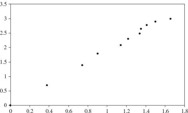
Figure IV.3.2 Log-log plot of holding period versus quantile ratio: $/£ forex rate

Table IV.3.2 Estimated scale exponents for $/£ forex rate and US interest rates

The US interest rates show evidence of trending, since the estimated scale exponent is greater than 0.5. Thus if mean reversion occurs, it does so over long periods and with a scale exponent of 0.6, scaling the 1% 1-day VaR on the US 3-month Treasury bill rate over a 10-day period implies an increase over the 1-day VaR of 10^0.6 rather than 10^0.5. In other words, the 1-day VaR of $1 million becomes $3.98 million over 10 days, rather than $3.16 million under square-root scaling.

Figure IV.3.3 Log-log plot of holding period versus quantile ratio: US 3-month Treasury bills

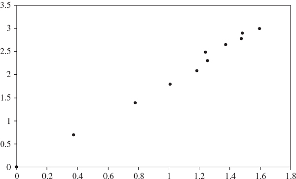
Figure IV.3.4 Log-log plot of holding period versus quantile ratio: US 10-year bond

In Tables IV.3.1 and IV.3.2 the estimated scale exponents were not identical when estimated at different quantiles. Either the variation is due to sampling error, or the distributions are not stable. In the next section we shall assume the variation is due to sampling error and use a scale exponent of 0.5 for the S&P 500 and the $/£ exchange rate,⁸ 0.55 for the US 10-year bond and 0.575 for the US 3-month Treasury bill.

It is commonly assumed that volatility scales with the square root of time, but we now show that this assumption may not be appropriate. Indeed, due to the rapid mean reversion of volatility, we should apply a scale exponent that is significantly less than 0.5. Table IV.3.3 summarizes the scale exponent on the S&P 500 volatility index (Vix), the FTSE 100 volatility index (Vftse) and the DAX 30 volatility index (Vdax) estimated using data since 1992.⁹ Scale exponent values estimated at an extreme quantile are very imprecise, but near-linear log-log plots are produced at the 5% quantile, and the spreadsheets accompanying this section imply that at this quantile the appropriate scale exponents are estimated at the values displayed in Table IV.3.3.

Table IV.3.3 Recommended scale exponents for volatility indices

Index	Scale exponent
Vix	0.355
Vftse	0.435
Vdax	0.425

IV.3.2.5 Scaling Historical VaR for Linear Portfolios

The returns on a linear portfolio are a weighted sum of returns on its assets or risk factors. If the returns on the assets or risk factors are stable, the portfolio returns will only be stable if all the assets or risk factors have the same scale exponents. In that case it makes no difference whether we scale the asset or risk factor returns before applying the portfolio mapping, or whether we apply the scaling to the portfolio returns directly. However, if the assets or risk factors have different scale exponents, which would normally be the case then the portfolio returns will not be stable.

To see this, consider the case of a portfolio, with weights w = (w₁,…, w_n) applied to n assets, and with daily log returns at time t denoted by x_t = (x_1t,…, x_nt)′. The daily log return on the portfolio at time t is then Y_1t = w′x_t. Now suppose the ith asset return is stable and has scale exponent . Then, the h-day log return on the portfolio is

unless λ = λ₁ = … = λ_n.

For instance, consider a portfolio for a UK investor with 50% invested in the S&P 500 index and 50% invested in the notional US 10-year bond. The S&P 500 and £/$ exchange rate returns may scale with the square root of the holding period, but the scale exponent for the US 10-year bond is approximately 0.55. Hence, the portfolio returns will not scale with the square root of the holding period.

We could therefore consider using one of the following approximations for scaling historical VaR, for a linear portfolio:

• Assume the assets or risk factor daily returns are stable, estimate their scale exponents, take an average and use this to scale them to h-day returns. Then apply the portfolio mapping to obtain the h-day portfolio returns.
• Alternatively, compute the portfolio daily returns, assume these are stable and estimate the scale exponent, then scale the portfolio's daily returns to h-day returns.

The first approach is the more approximate of the two, but it has distinct practical advantages over the second approach. First, the analyst may store a set of estimated scale exponents for the major risk factors, in which case there is no need to re-estimate a scale exponent for each and every portfolio. Secondly, returns on major risk factors may be more likely to have stable distributions than arbitrary portfolios. The advantage of the second approach is that it should produce more accurate scaling rules, possibly with scale exponents depending on the significance levels for VaR, but its disadvantage is that a very large historical sample of portfolio returns is required if the scale exponents are to be measured accurately, particularly for extreme quantiles.

IV.3.2.6 Errors from Square-Root Scaling of Historical VaR

Any deviation from square-root scaling is of particular interest for economic capital allocation, where extreme quantiles such as 0.1% may be scaled over long horizons. Table IV.3.4 displays the h-day VaR that is scaled up from the 1-day VaR of $1 million, for different risk horizons h and for different values of the scale exponent. The square-root scaling rule gives the VaR estimates in the centre column (shown in bold). For instance, with square-root scaling a 1-day VaR of $1 million would scale to $10^0.5 million, i.e. $3.16 million over 10 days. The other columns report the VaR based on other scale exponents, expressed as a percentage of this figure. For instance, if the scale exponent were 0.6 instead of 0.5, the 1-day VaR would scale to 1.259 × $3.16 million, i.e. $3.978 million over 10 days.

Table IV.3.4 Scaling 1-day VaR for different risk horizons and scale exponents

If we applied a square-root scaling rule, when a power law scaling with a different exponent is in fact appropriate, the errors could be very large indeed. When the scale exponent is greater than 0.5 the square-root scaling law may substantially underestimate VaR and when it is greater than 0.5 the square-root scaling law may substantially overestimate VaR, especially for long term risk horizons. Given the scale exponents for major risk factors that were estimated in Section IV.3.2.4, using a square-root scaling rule is about right for the VaR on US equities and the £/$ exchange rate, but it would substantially underestimate the VaR on US interest rates. And when volatility is a risk factor, square-root scaling of a positive vega exposure would lead to a very considerable overestimation of VaR, because volatility mean-reverts rapidly.

IV.3.2.7 Overlapping Data and Multi-Step Historical Simulation

Historical scenarios capture the empirical dependencies between risk factors in a natural way, just by sampling contemporaneous historical returns on each risk factor. Multi-step historical scenarios can also capture the dynamic behaviour in each risk factor, such as volatility clustering, just by simulating consecutive returns in the order they occurred historically. For a linear portfolio, multi-step simulation consists of simulating an h-day log return by summing h consecutive daily log returns, and only then revaluing the portfolio. By contrast, for a portfolio of path-dependent products, we would need to evaluate the portfolio on every consecutive day over the risk horizon, which can be very time-consuming.

Unless we also apply a parametric model, as in the filtered historical simulation model described in Section IV.3.3.4, multi-step historical simulation presents a problem if we use overlapping samples, because this can distort the tail of the return distribution. To see why, suppose we observe 1000 daily P&Ls that are normal and i.i.d. with zero mean. Suppose that, by chance, these are all relatively small, i.e. of the order of a few thousand US dollars, except for one day when there was a very large negative P&L of $1 million. Then $1 million is the 0.1% daily VaR. However, the 1% daily VaR is much smaller. Let us assume it is $10,000, so that VaR_1,0.1% is 100 times larger than VaR_1,1%. What can we say about the 10-day VaR at these significance levels?

Since the daily returns are normal and i.i.d. we may scale VaR using the square-root-of-time rule. Thus, VaR_10,0.1% will be 100 times larger than VaR_10,1%. In other words, using the square-root-of-time rule, the loss that is experienced once every 40 years is 100 times the loss that is experienced once every 4 years.

Now consider the 10-day P&L on the same variable. When based on non-overlapping data there are 100 observations, only one of which will be about $1 million. So the 1% 10-day VaR is about $1 million, which is much larger than it would be using the square-root scaling rule. And the 0.1% 10-day VaR cannot be measured because there are not enough data. However, we might consider using overlapping 10-day P&Ls, so that we now have 1000 observations and 10 of these will be approximately $1 million. Then the 1% 10-day VaR is again about $1 million, and now we can measure the 0.1% 10-day VaR – and it will also be about $1 million! So, using overlapping data, the loss that is experienced once every 40 years is about the same as the loss that is experienced once every 4 years. That is, the 0.1% 10-day VaR is about the same as the 1% 10-day VaR. In short, using overlapping data in this way will distort the lower tail of the P&L distribution, creating a tail that is too ‘blunt’ below a certain quantile, i.e. the 1% quantile in this exercise.

Thus, to apply multi-step historical simulation for estimating h-day VaR without distorting the tails, one has to apply some type of filtering, such as method described in Section IV.3.3.4. However, we do not necessarily need to apply multi-step simulation. Under certain assumptions about risk factor returns and the portfolio's characteristics, we can scale up the daily VaR to obtain an h-day VaR estimate, as described in the previous subsections.

IV.3.3 IMPROVING THE ACCURACY OF HISTORICAL VALUEATRISK

This section begins with a case study which demonstrates that the historical VaR based on an equally weighted return distribution depends critically on the choice of sample size. In fact, when data are equally weighted it is our choice of sample size, more than anything else, that influences the VaR estimate. By showing how close the normal linear VaR and historical VaR estimates are to each other, we show that the sample size is the most important determinant of the VaR estimate. The main learning point of this case study is that equal weighting of risk factor returns is not advisable for any VaR model.

In the linear and Monte Carlo VaR models the risk factor returns data are summarized in a covariance matrix, and instead of equally weighted returns this matrix can be constructed using an exponentially weighted moving average model. But, if not equal, what sort of weighting of the data should we use in historical VaR? After the case study we describe two different ways of weighting the risk factor returns data before the distribution of the portfolio returns is constructed: exponential weighting of probabilities and volatility adjustment of returns. Volatility adjustment motivates the use of filtered historical simulation, described in Section IV.3.3.4.

IV.3.3.1 Case Study: Equally Weighted Historical and Linear VaR

For a given portfolio the historical and normal linear VaR estimates based on the same sample are often much closer than two historical VaR estimates based on very different samples. We demonstrate this with a case study of VaR estimation for a simple position on the S&P 500 index. Figure IV.3.5 shows the daily historical prices of the S&P 500 index (in black) and its daily returns (in grey) between 31 December 1986 and 31 March 2008. The effects of the Black Monday stock market crash in October 1987, the Russian crisis in August 1998, the technology boom in the late 1990s and subsequent bubble burst in 2001 and 2002, and the US sub-prime mortgage crisis are all evident.

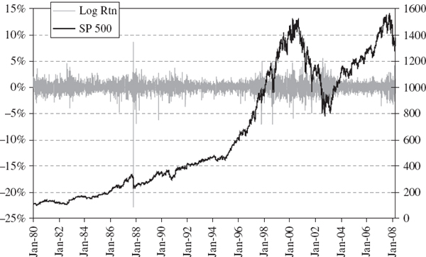
Figure IV.3.5 S&P 500 index and daily returns

In the case study we:

• apply both the normal linear and the historical VaR models to estimate VaR for a single position on the S&P 500 index, using an equally weighted standard deviation in the normal linear model and an equally weighted return distribution in the historical simulation model;
• compare time series of the two VaR estimates over a 1-day horizon at the 99% confidence level;¹⁰
• compare time series of VaR estimates over a rolling data window based on a sample of size T = 500 and of T = 2000 data points.

Hence, two time series of VaR estimates are computed, for each choice of T, using a quantile estimated from the histogram of returns for the historical simulation model and an equally weighted standard deviation for the normal linear VaR. All figures are expressed as a percentage of the portfolio value.

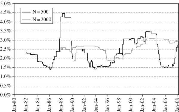
Figure IV.3.6 Time series of 1% historical VaR estimates, S&P 500

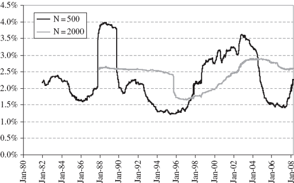
Figure IV.3.7 Time series of 1% normal linear VaR estimates, S&P 500

Figures IV.3.6 and IV.3.7 display the time series of 1-day 1% VaR estimates obtained from each model, starting in December 1981 for T = 500 and starting in December 1987 for T = 2000. For each estimate we use the T most recent daily returns. The VaR based on 500 observations is, of course, more variable over time than the VaR based on 2000 observations, since we are weighting all the data equally. The ‘ghost effect’ of the 1987 global crash is evident in both graphs, particularly so in the VaR based on 500 observations. Then, exactly 500 days after the crash – and even though nothing particular happened on that day – the VaR returned to more normal levels. Most of the time the historical VaR is dominated by a few extreme returns, even when the sample contains 2000 observations, and when one of these enters or leaves the data set the VaR can exhibit a discrete jump upward or downward.¹¹

Notice that the two different historical VaR estimates based on N = 500 and N = 2000 differ by 1%–2% on average. The two normal linear VaR estimates have differences of a similar magnitude, though slightly smaller in general. In fact, there is more similarity between the normal and historical VaR estimates for a fixed sample size than there is between the historical VaR estimates for different sample sizes! Figure IV.3.8 shows that the historical VaR tends to be slightly greater than the normal linear VaR, and this is expected due to the excess kurtosis in the S&P 500 daily return distribution.¹² This figure shows that, on average, the historical VaR is about 0.2% (of the portfolio value) greater than the normal linear VaR.¹³

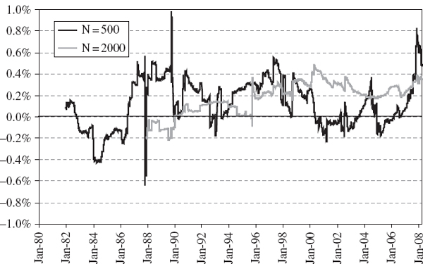
Figure IV.3.8 Time series of difference between historical VaR and normal linear VaR, S&P 500

The global equity crash of 1987 is a major stress event in the sample: the S&P 500 fell by 23% in one day between 18 and 19 October 1987. This single return had a very significant impact on the normal linear VaR estimate because the equally weighted volatility estimate (based on the last 500 days) jumped up almost 7 percentage points, from 15.6% on 18 October to 22.5% on 19 October. However, this single initial return of the global equity crash had much less effect on the historical VaR: it was just another return in the lower tail and its huge magnitude was not taken into account. So on 19 October 1987, the normal linear VaR rose more than 1% overnight, whilst the historical VaR rose by only 0.03% of the portfolio value. It was not until we had experienced several days of large negative returns that the historical VaR ‘caught up’ with the normal linear VaR. Hence in Figure IV.3.8 we see a short period in October 1987 when the normal linear VaR was about 0.6% (of the portfolio value) above the historical VaR estimate. Then, exactly 500 days later, when the global crash data falls out of the sample, the normal linear VaR jumps down as abruptly as it jumped up, whilst the historical VaR takes a few days to decrease to normal levels. So in Figure IV.3.8, during October 1989, we see a short period where the historical VaR is much greater than the normal linear VaR.

We conclude that when returns data are equally weighted it is the sample size, rather than the VaR methodology, that has the most significant effect on the error in the VaR estimates. Clearly, equal weighting of returns data causes problems in all VaR models. Any extreme market movement will have the same effect on the VaR estimate, whether it happened years ago or yesterday, provided that it still occurs during the sample period. Consequently the VaR estimate will suffer from ‘ghost features’ in exactly the same way as equally weighted volatility or correlation estimates. Most importantly, when data are equally weighted, the VaR estimate will not be sufficiently risk sensitive, i.e it will not properly reflect the current market conditions. For this reason both the parametric linear and historical VaR models should apply some type of weighting to the returns data, after which ghost features are no longer so apparent in the VaR estimates.

IV.3.3.2 Exponential Weighting of Return Distributions

A major problem with all equally weighted VaR estimates is that extreme market events can influence the VaR estimate for a considerable period of time. In historical simulation, this happens even if the events occurred long ago. With equal weighting, the ordering of observations is irrelevant. In Chapter II.3 we showed how this feature also presents a substantial problem when equally weighted volatilities and correlations are used in short-term forecasts of portfolio risk, and that this problem can be mediated by weighting the returns so that their influence diminishes over time.

To this end, Section II.3.8 introduced the exponentially weighted moving average methodology. We applied EWMA covariance matrices in the normal linear VaR model in Section IV.2.10. In Section IV.2.10.1 we showed that a EWMA covariance matrix may be thought of as an equally weighted covariance matrix on exponentially weighted returns, where each return is multiplied by the square root of the smoothing constant λ raised to some power n, where n is the number of days since the observed return occurred. After weighting the returns in this way, we apply equal weighting to estimate the variances and covariances.

The historical VaR model can also be adapted so that it no longer weights data equally. But instead of multiplying the portfolio returns by the square root of the smoothing constant raised to some power, we assign an exponential weight to the probability of each return in its distribution.¹⁴ Fix a smoothing constant, denoted λ as usual, between 0 and 1. Then assign the probability weight 1 − λ to the most recent observation on the return, the weight λ (1 − λ) to the return preceding that, and then weights of λ²(1 − λ ), λ³ (1 − λ ), λ⁴ (1 − λ ),… as the observations move progressively further into the past. When the weights are assigned in this way, the sum of the weights is 1, i.e. they are probability weights.

Figure IV.3.9 shows the weights that would be assigned to the return on each day leading up to the time that the VaR is measured, for three different values of λ, i.e. 0.999, 0.99 and 0.9. The horizontal axis represents the number of days before the VaR is measured. The larger the value of λ, the lower the weight on recent returns and the higher the weight assigned to returns far in the past.

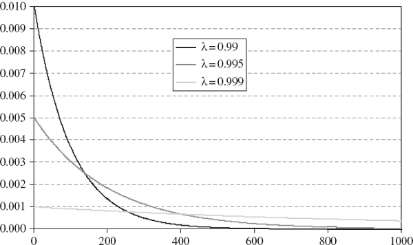
Figure IV.3.9 Exponential probability weights on returns

Then we use these probability weights to find the cumulative probability associated with the returns when they are put in increasing order of magnitude. That is, we order the returns, starting at the smallest (probably large and negative) return, and record its associated probability weight. To this we add the weight associated with the next smallest return, and so on until we reach a cumulative probability of 100α%, the significance level for the VaR calculation. The 100α% historical VaR, as a percentage of the portfolio's value, is then equal to minus the last return that was taken into the sum. The risk horizon for the VaR (before scaling) is the holding period of the returns, i.e. usually 1 day.

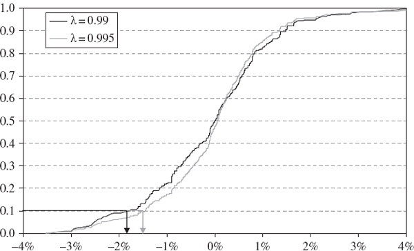
Figure IV.3.10 shows the cumulative probability assigned to the S&P 500 empirical return distribution, based on the 1000 daily returns prior to 31 March 2008, the time when the VaR is measured. We use the same data as for the case study in the previous section, starting on 6 April 2004. For a given λ, start reading upward from the lowest daily return of −3.53% (which occurred on 27 February 2007) adding the exponentially weighted probability associated with each return as it is included. The α quantile return is the one that has a cumulative probability of α associated with it.

Figure IV.3.10 Exponentially weighted distribution functions, S&P 500 daily returns

The quantiles depend on the value chosen for the weighting constant λ. The 10% quantiles are indicated on Figure IV.3.10 for λ = 0.99 and 0.995.¹⁵ From these we see immediately that the 10% VaR, which is minus the 10% quantile, is approximately 1.7% when λ = 0.99 and approximately 1.45% when λ = 0.995. But when λ = 0.999 the 10% VaR, not shown in Figure IV.3.10, is approximately 3%. Hence, the VaR does not necessarily increase or decrease with λ. It depends on when the largest returns occurred. If all the largest returns occurred a long time before the VaR is estimated, then higher values of lambda would give a larger VaR estimate. Otherwise, it is difficult to predict how the VaR at different quantiles will behave as λ varies. The problem with this methodology is that the choice of λ (which has a very significant effect on the VaR estimate) is entirely ad hoc.

IV.3.3.3 Volatility Adjustment

One problem with using data that span a very long historical period is that market circumstances change over time. Equity markets go through periods of relatively stable, upward-trending prices, periods of range bounded price behaviour, and periods where prices fall rapidly and (often) rebound. Commodity futures markets may be exposed to bubbles, seasonal price fluctuations and switching between backwardation and contango.¹⁶ Currency market volatility comes in clusters and is influenced by government policy on intervention. Fiscal policy also varies over the business cycle, so the term structures of interest rates and the prices of interest rate sensitive instruments shift between different behavioural regimes. In short, regime specific economic and behavioural mechanisms are a general feature of financial markets.

Since historical simulation requires a very large sample, this section addresses the question of how best to employ data, possibility from a long time ago when the market was in a different regime. As a simple example, consider an equity market that has been stable and trending for one or two years, but previously experienced a long period of high volatility. We have little option but to use a long historical sample period for the historical VaR estimate, but we would like to adjust the returns from the volatile regime so that their volatility is lower. Otherwise the current historical VaR estimate will be too high. Conversely, if markets are particularly volatile at the moment but were previously stable for many years, an unweighted historical estimate will tend to underestimate the current VaR, unless we scale up the volatility of the returns from the previous, tranquil period.

We now consider a volatility weighting method for historical VaR that was suggested by Duffie and Pan (1997) and Hull and White (1998). The methodology is designed to weight returns in such a way that we adjust their volatility to the current volatility. To do this we must obtain a time series of volatility estimates for the historical sample of portfolio returns. The best way to generate these would be to use an appropriate asymmetric GARCH model, as described in Section II.4.3, although a simple EWMA model may also be quite effective.¹⁷

Denote the time series of unadjusted historical portfolio returns by and denote the time series of the statistical (e.g. GARCH or EWMA) volatility of the returns by , where T is the time at the end of the sample, when the VaR is estimated. Then the return at every time t < T is multiplied by the volatility estimated at time T and divided by the volatility estimated at time t. That is, the volatility adjusted returns series is

where T is fixed but t varies over the sample, i.e. {t = 1,…, T}. A time-varying estimate of the volatility of the series (IV.3.3), based on the same model that was used to obtain _t, should be constant and equal to _T, i.e. the conditional volatility at the time the VaR is estimated.¹⁸

EXAMPLE IV.3.1: VOLATILITY ADJUSTED VAR FOR THE S&P 500 INDEX

Use daily log returns on the S&P 500 index from 2 January 1995 to 31 March 2008 to estimate symmetric and asymmetric GARCH volatilities. For each time series of volatility estimates, plot the volatility adjusted returns that are obtained using (IV.3.3), where the fixed time T is 31 March 2008, i.e. the date that the VaR is estimated. Then find the 100α% 1-day historical VaR estimate, as a percentage of the portfolio value, based on both of the volatility adjusted series. For α = 0.001, 0.01, 0.05 and 0.1 compare the results with the unadjusted historical VaR.

SOLUTION The GARCH estimates are obtained using the Excel spreadsheet.¹⁹ Table IV.3.5 displays the estimated parameters of the two GARCH models.²⁰

Table IV.3.5 GARCH parameters for S&P 500 index

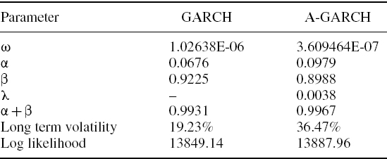
There is a leverage effect in the A-GARCH model, which captures the asymmetric response of volatility to rises and falls in the index. The index has many significant falls during the sample period, each one precipitating a higher volatility than a rise in the index of the same magnitude. The symmetric GARCH volatility ignores this effect, and hence underestimates the long term average index volatility over the sample. This is about 20% according to the GARCH model, but over 36% according to the A-GARCH model.

Also, compared with the A-GARCH volatility the symmetric GARCH volatility shows less reaction to market events (because α is smaller) but greater persistence following a market shock (because β is greater). The log likelihood will always be higher in the asymmetric GARCH model, since it has one extra parameter. Nevertheless it is still clear that capturing an asymmetric volatility response greatly improves the fit to the sample data in this case.

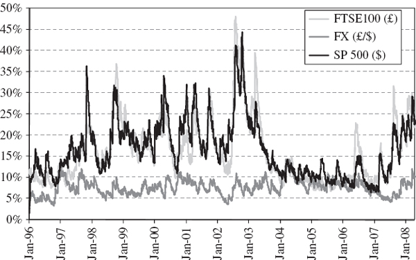
The resulting GARCH volatility estimates are compared in Figure IV.3.11. This shows that the index volatility varied considerably over the sample period, reaching highs of over 45% during the Asian crisis in 1997, the Russian crisis in 1998 and after the burst of the technology bubble. The years 2003–2006 were very stable, with index volatility often as low as 10% and only occasionally exceeding 15%, but another period of market turbulence began in 2007, precipitated by the credit crisis.

We now calculate the volatility adjusted returns that form the basis of the empirical distribution from which the historical VaR is computed as a quantile. Figure IV.3.12 illustrates the A-GARCH volatility adjusted returns, and compares them with the unadjusted returns. Before adjustment, volatility clustering in returns is evident from the change in magnitude of the returns over the historical period. For instance, the returns during the years 2003–2006 were considerably smaller, on the whole, than the returns during 2002. But after adjustment the returns have a constant volatility equal to the estimated A-GARCH volatility at the end of the sample.

Now we estimate the 1% 1-day historical VaR for a position on the S&P 500 index on 31 March 2008, based on the unadjusted returns and based on the volatility adjusted returns (IV.3.3) with both the symmetric and the asymmetric GARCH volatilities. The results, reported in Table IV.3.6, indicate a considerable underestimation of VaR when the returns are not adjusted.²¹

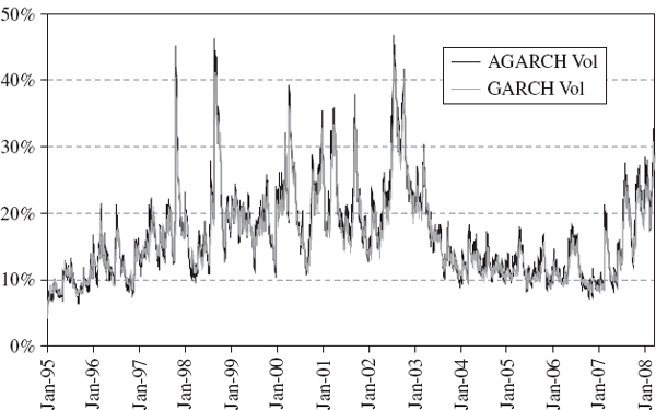
Figure IV.3.11 GARCH volatility estimates for the S&P 500 index

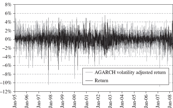
Figure IV.3.12 Returns and A-GARCH volatility adjusted returns

The above example demonstrates how volatility adjustment compares favourably with the exponential weighting method in the previous section. The main advantages of using a GARCH model for volatility adjustment are as follows:

• We do not have to make a subjective choice of an exponential smoothing constant λ. The parameters of the GARCH model may be estimated optimally from the sample data.
• We are able to use a very large sample for the return distribution. In the above example we used 3355 returns, and an even larger sample would also be perfectly feasible.

Table IV.3.6 Historical VaR for S&P 500 on 31 March 2008

Hence this type of volatility adjustment allows the VaR at very high quantiles to be estimated reasonably accurately.

We end this subsection by investigating the effect of volatility adjustment on the scale exponent that we might use to transform a 1-day historical VaR estimate into an h-day historical VaR estimate. However, in the next subsection we shall describe a more sophisticated method for computing h-day historical VaR, which uses a dynamic model, such as the GARCH volatility adjustment models described above, and does not require the use of power law scaling.

Recall that to estimate the values of the scale exponent shown in Table IV.3.1, over 50 years of daily returns on the S&P 500 were used. We now scale these returns to have constant volatility, using (IV.3.3), this time using a simple EWMA volatility instead of a GARCH model. It does not matter which volatility level we scale the series to, the estimated scale exponent remains unchanged.²² Table IV.3.7 reports the results, which are computed in an Excel workbook in the case study folder for this subsection. They are calculated in a similar way to the unadjusted scale exponents in Table IV.3.1, but now the results are presented using different values for the smoothing constant rather than different sample sizes.

Table IV.3.7 Estimated values of scale exponent for volatility adjusted S&P 500

In this subsection we have considered volatility adjustment at the portfolio level. That is, we construct a returns series for the portfolio in the usual way, and then adjust this to have the required volatility. Later in this chapter, in Section IV.3.5.2, we show how to volatility-adjust individual risk factors for a portfolio, and we use a case study to compare the VaR based on volatility adjustment at the risk factor level with the VaR based on portfolio level volatility adjustment.

IV.3.3.4 Filtered Historical Simulation

Barone-Adesi et al. (1998, 1999) extend the idea of volatility adjustment to multi-step historical simulation, using overlapping data in a way that does not create blunt tails for the h-day portfolio return distribution. Their idea is to use a parametric dynamic model of returns volatility, such as one of the GARCH models that were used in the previous subsection, to simulate log returns on each day over the risk horizon.

For instance, suppose we have estimated a symmetric GARCH model on the historical log returns r_t, obtaining the estimated model

The filtered historical simulation (FHS) model assumes that the GARCH innovations are drawn from the standardized empirical return distribution. That is, we assume the standardized innovations are

where r_t is the historical log return and _t is the estimated GARCH daily standard deviation at time t.

To start the multi-step simulation we set ₀ to be equal to the estimated daily GARCH standard deviation on the last day of the historical sample, when the VaR is estimated, and also set r₀ to be the log return on the portfolio from the previous day to that day. Then we compute the GARCH daily variance on day 1 of the risk horizon as

Now the simulated log return on the first day of the risk horizon is ₁ = ∈₁₁ where a value for ∈₁ is simulated from our historical sample of standardized innovations (IV.3.5). This is achieved using the statistical bootstrap, which is described in Section I.5.7.2. Thereupon we iterate in the same way, on each day of the risk horizon setting

where ∈_t is drawn independently of ∈_t−1 in the bootstrap. Then the simulated log return over a risk horizon of h days is the sum ₁ + ₂ +… + _h. Repeating this for thousands of simulations produces a simulated return distribution, and the 100α% h-day FHS VaR is obtained as minus the α quantile of this distribution.

We do not need to use a symmetric GARCH model for the filtering. In fact, the next example illustrates the FHS method using the historical data and the estimated A-GARCH model from the previous example.

EXAMPLE IV.3.2: FILTERED HISTORICAL SIMULATION VAR FOR THE S&P 500 INDEX

Use daily log returns on the S&P 500 index from 2 January 1995 to 31 March 2008 to estimate the 100α% 10-day VaR using FHS based on an asymmetric GARCH model with the parameters shown in Table IV.3.5. For α = 0.001, 0.01, 0.05 and 0.1 compare the results with the asymmetric GARCH volatility adjusted historical VaR that is obtained by scaling up the daily VaR estimates using a square-root scaling rule.

SOLUTION The starting values are taken from the results in Example IV.6.1: the A-GARCH annual volatility on 31 March 2008, when the VaR is estimated, is 27.82% and the daily log return on 31 March 2008 is 0.57%. Then each daily log return over the risk horizon is simulated by taking the current A-GARCH estimated standard deviation and multiplying this by an independent random draw from the standardized empirical returns.²³ The results from one set of 5000 simulations are shown in the second column of Table IV.3.8. The third column, headed ‘scaled volatility adjusted VaR’, is obtained by multiplying the results in the last column of Table IV.3.6 by . The results vary depending on the simulation, but we almost always find that the FHS 10-day VaR is just slightly lower than the volatility adjusted VaR based on square-root scaling up of the daily VAR for every quantile shown.

Table IV.3.8 Scaling VaR versus filtered historical simulation

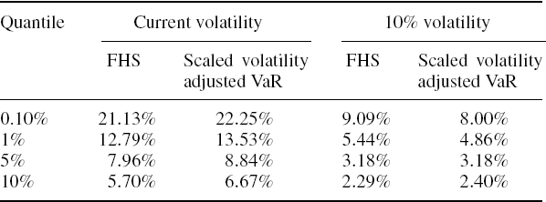
Now suppose the current A-GARCH volatility were only 10% instead of 27.82%. Readers can change the starting value in cell D3 of the spreadsheet to 0.6325%, i.e. the daily standard deviation corresponding to 10% volatility, and see the result. The results from one set of 5000 filtered historical simulations are shown in the fourth column of Table IV.3.8 and the scaled up volatility adjusted VaR corresponding to 10% volatility is shown in the last column. Now, more often than not, the FHS VaR is greater than the scaled volatility adjusted daily VaR at the extreme quantiles but not, for instance, at the 10% quantile. Why is this so?

Looking again at Figure IV.3.11, we can see that the average level of volatility over our historical sample was below 20%. In fact, the average estimated A-GARCH volatility was 16.7% over the sample. So on 31 March 2008 the volatility was higher than average and in the absence of an extreme return during the risk horizon it would revert toward the long term average, as GARCH volatilities do, which in this case entails reverting downward. By contrast, the 10% volatility is below average so it will start reverting upward toward 16.7% over the risk horizon, in the absence of an extreme return during this period.

But there is no mean reversion in a square-root scaling of daily VaR. Indeed, this type of scaling is theoretically incorrect when we use a GARCH model for volatility adjustment.²⁴ It assumes the volatility remains constant over the risk horizon and does not mean-revert at all. Square-root scaling corresponds to an i.i.d. normal assumption for returns, which certainly does not hold in the FHS framework. Hence, when adjustment is made using a GARCH model, the scaled volatility adjusted VaR will overestimate VaR when the current volatility is higher than average, and underestimate VaR when volatility is lower than average.

IV.3.4 PRECISION OF HISTORICAL VALUE AT RISK AT EXTREME QUANTILES

When using very large samples and measuring quantiles no more extreme than 1%, the volatility adjustment and filtering described in the previous section are the only techniques required. For daily VaR you just need to estimate the required quantile from the distribution of the volatility adjusted daily portfolio returns, as described in Section IV.3.3.3. And when VaR is estimated over horizons longer than 1 day, apply the filtering according to your volatility adjustment model, as described in Section IV.3.3.4.

But it may be necessary to compute historical VaR at very extreme quantiles when it is impossible to obtain a very large sample of historical returns on all assets and risk factors. For instance, economic capitalization at the 99.97% confidence level is a target for most firms with a AA credit rating, but it is impossible to obtain reliable estimates of 0.03% VaR directly from a historical distribution, even with a very large sample indeed.

To assess historical VaR at very extreme quantiles – and also at the usual quantiles when the sample size is not very large – one needs to fit a continuous distribution to the empirical one, using a form that captures the right type of decay in the tails. This section begins by explaining how kernel fitting can be applied to the historical distribution without making any parametric assumption about tail behaviour. We then consider a variety of parametric or semi - parametric techniques that can be used to estimate historical VaR at extreme quantiles.

IV.3.4.1 Kernel Fitting

In Section I.3.3.12 we explained how to estimate a kernel to smooth an empirical distribution. Having chosen a form for the kernel function, the estimation algorithm fits the kernel by optimizing the bandwidth, which is like the cell width in a histogram. Fitting a kernel to the historical distribution of volatility adjusted returns allows even high quantiles to be estimated from relatively small samples. The choice of kernel is not really important, as shown by Silverman (1986), provided only that a reasonable one is chosen. For empirical applications of kernel fitting to VaR estimation see Sheather and Marron (1990), Butler and Schachter (1998) and Chen and Tang (2005).

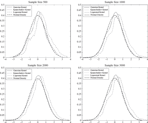
To illustrate this we use Matlab to apply the Epanechnikov, Gaussian and lognormal kernels to a distribution of volatility adjusted returns shown in Figure IV.3.13. This series is of daily returns on the S&P 500 index, and the volatility adjustment has been made using a EWMA volatility with smoothing constant 0.95. We fit a kernel to a sample size of 500, 1000, 2000 and 3000 returns. In each case the returns are standardized to have mean 0 and variance 1 before fitting the kernel. Figure IV.3.14 compares the three kernel densities with the standard normal density to give a visual representation of the skewness and excess kurtosis in the empirical densities. Whilst the Gaussian and Epanechnikov kernels are almost identical, the lognormal kernel fits the data very badly indeed.

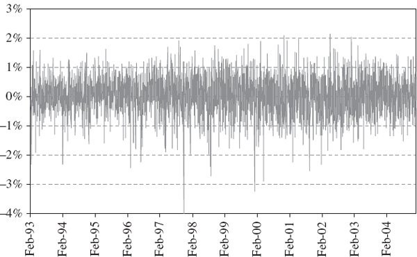
Figure IV.3.13 EWMA adjusted daily returns on S&P 500

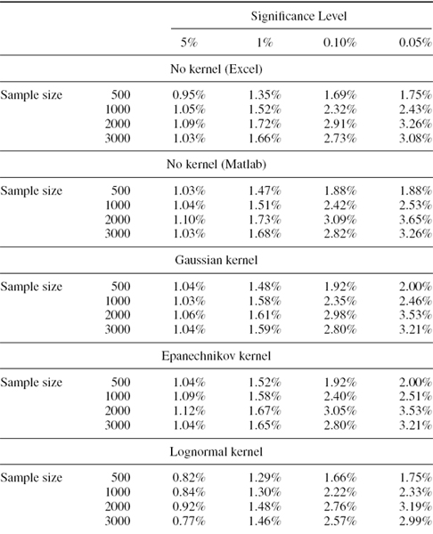
Now without fitting a kernel, and for each fitted kernel, we estimate the 1-day VaR at 5%, 1%, 0.1% and 0.05% significance levels. The results are shown in Table IV.3.9 and, as usual, they are expressed as a percentage of the portfolio value. Note that there are two sets of results labelled ‘No kernel’: the first uses the Excel PERCENTILE function, which we know has some peculiarities;²⁵ and the second uses the Matlab quantile function which is more accurate than that of Excel.²⁶

As remarked above, the lognormal kernel provides a poor fit and so the results should not be trusted. Whilst the VaR results for the Gaussian and Epanechnikov kernels are very similar (they are identical in exactly one-half of the cases) those for the lognormal kernel are very different and are very far from the quantiles that are calculated by Excel and Matlab. The Matlab quantiles estimate the VaR fairly accurately; in fact, the results are similar to those obtained using the Gaussian and Epanechnikov kernels. However, there is a marked difference between these and the quantiles estimated using the Excel function.

Another feature of the results in Table IV.3.9 is that the VaR estimates are sample-specific. The sample of the most recent 2000 returns clearly has heavier tails than the sample of the most recent 3000 returns or the sample of the most recent 1000 returns, since the VaR estimates are greatest when based on a sample size 2000.

Figure IV.3.14 Kernels fitted to standardized historical returns

IV.3.4.2 Extreme Value Distributions

Kernel fitting is a way to smooth the empirical returns density whilst fitting the data as closely as possible. A potential drawback with this approach is that the particular sample used may not have tails as heavy as those of the population density. An alternative to kernel fitting is to select a parametric distribution function that is known to have heavy tails, such as one of the extreme value distributions. Then we fit this either to the entire return distribution or to only the observations in some pre-defined lower tail. A generalized extreme value (GEV) distribution can be fitted to the entire empirical portfolio return distribution, but the generalized Pareto distribution (GPD) applies to only those returns above some pre-defined threshold u.

Another potential drawback with kernel fitting is that it does not lend itself to scenario analysis in the same way as parametric distribution fitting. When a parametric form is fitted to the returns it is possible to apply scenarios to the estimated parameters to see the effect on VaR. For instance, having estimated the scale and tail index parameters of a GPD from the historical returns over some threshold, alternative VaR estimates could be obtained by changing the scale and tail index parameters.²⁷ For instance, we might fit the GPD to only those returns in the lower 10% tail of the distribution. Provided that the historical sample is sufficiently large (at least 2000 observations), there will be enough returns in the 10% tail to obtain a reasonably accurate estimate of the GPD scale and tail index parameters, β and ξ.

Table IV.3.9 Historical VaR based on kernel fitting

It can be shown that when a GPD is fitted to losses in excess of a threshold u there is a simple analytic formula for the 100α%VaR,

where n is the number of returns in the entire sample and n_u is the number of returns less than the threshold u. It is therefore simple to generate VaR estimates for different values of β and ξ.

EXAMPLE IV.3.3: USING THE GPD TO ESTIMATE VAR AT EXTREME QUANTILES

Estimate the parameters of a GPD for the EWMA volatility adjusted daily returns on the S&P 500 that were derived and analysed in Section IV.3.4.1. Base your results on the entire sample of 14,264 returns and also on a sample of the 5000 most recent returns. In each case set the volatility in the adjusted returns to be 10%.²⁸ Use only the returns that are sampled below a threshold of (a) 20%, (b) 10%, (c) 5% and (d) 1%. Hence, estimate the 1-day VaR using (IV.3.6) and compare the results with the historical VaR that is estimated without fitting a GPD. In each case use a risk horizon of 1 day and confidence levels of 99%, 99.9% and 99.95%, and express the VaR as a percentage of the portfolio value.

SOLUTION The returns are first normalized by subtracting the sample mean and dividing by the standard deviation, so that they have mean 0 and variance 1. Then for each choice of threshold, the GPD parameters are estimated using maximum likelihood in Matlab.²⁹ The results are reported in the two columns headed ‘GPD parameters’ in Table IV.3.10.

Table IV.3.10 Estimates of GPD parameters (Matlab)

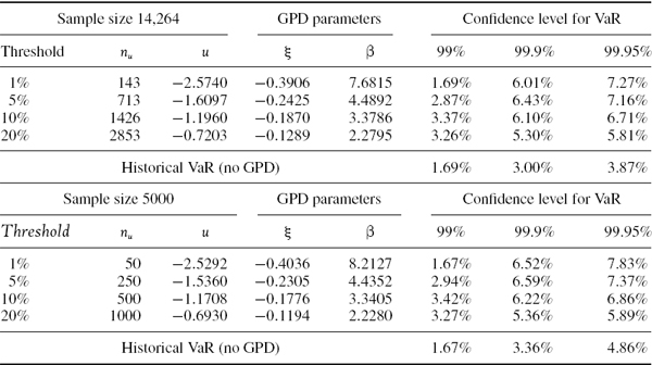
Since our GPD parameters were estimated on the normalized returns, after we compute the VaR using (IV.3.6) we must then de-normalize the VaR estimate, i.e. multiply it by the standard deviation and subtract the mean. This gives the results shown in Table IV.3.10 under the three columns headed ‘Confidence level for VaR’. The GPD results should be compared to the historical VaR without fitting a GPD, i.e. the VaR that is estimated from a quantile of the volatility adjusted return distribution. This is shown in the last row of each half of the table.

The GPD VaR is greater than the volatility adjusted VaR that is obtained without the GPD fit, and substantially so for extreme quantiles. For instance, at the 0.05% quantile and based on the most recent 5000 returns, the GPD VaR based on a threshold of 10% is 6.86% of the portfolio value, whereas the historical VaR without fitting the GPD is estimated to be only 4.86% of the portfolio value.

Notice how the historical VaR that is obtained without fitting the GPD is greatly influenced by the sample size. Even after the volatility adjustment, 5000 returns are simply insufficient to estimate VaR at the 99.95% confidence level with accuracy. At this level of confidence we are looking for a loss event that has no more than 1 chance in 2000 of occurring.

The GPD VaR estimates are not greatly influenced by the sample size, but they are influenced by the choice of threshold. A threshold of 10% or 20% is adequate, but for thresholds of 5% and 1% there is insufficient data in the tail to fit the GPD parameters accurately starting with a sample size of 5000.³⁰

An important point to learn from this example is that although the GPD VaR estimates are fairly robust to changes in sample size, they are not robust to the choice of threshold. This is one of the disadvantages of using the GPD to estimate VaR, since the choice of threshold is an important source of model risk. Advocates of GPD VaR argue that this technique allows suitably heavy tails to be fitted to the data, and so it is possible to estimate historical VaR at very high confidence levels such as 99.97%. Another convenient aspect of the approach is that the expected tail loss (also called the conditional VaR) has a simple analytic form, which we shall introduce in Section IV.3.7.2.

IV.3.4.3 Cornish–Fisher Approximation

The Cornish–Fisher expansion (Cornish and Fisher, 1937) is a semi-parametric technique that estimates quantiles of non-normal distributions as a function of standard normal quantiles and the sample skewness and excess kurtosis. In the context of historical VaR, this technique allows extreme quantiles to be estimated from standard normal quantiles at high significance levels, given only the first four moments of the portfolio return or P&L distribution.

The fourth order Cornish–Fisher approximation _α to the α quantile of an empirical distribution with mean 0 and variance 1 is

where z_α = Φ⁻¹(α) is the α quantile of a standard normal distribution, and and denote the skewness and excess kurtosis of the empirical distribution. Then, if and denote the mean and standard deviation of the same empirical distribution, this distribution has approximate α quantile

EXAMPLE IV.3.4: CORNISH–FISHER APPROXIMATION

Find the Cornish–Fisher approximation to the 1% quantile of an empirical distribution with the sample statistics shown in Table IV.3.11. Then use this approximation to estimate the 1% 10-dayVaR based on the empirical distribution, and compare this with the normal linear VaR.

Table IV.3.11 Sample statistics used for Cornish–Fisher approximation

Annualized mean	5%
Annualized standard deviation	10%
Skewness	−0.6
Excess kurtosis	3

SOLUTION The normal linear VaR estimate is

To calculate the Cornish–Fisher VaR we first ignore the mean and standard deviation, and apply the expansion (IV.3.7) to approximate the 1% quantile of the normalized distribution having zero mean and unit variance.

Since z_0.01 = Φ⁻¹(0.01) = − 2.32635 we have , so using (IV.3.7),³¹

The mean and variance over the risk horizon are 0.2% and 2%, so (IV.3.8) becomes

Hence, based on the Cornish-Fisher expansion, the 1% 10-day VaR is 6.47% of the portfolio value, compared with 4.65% for the normal linear VaR.

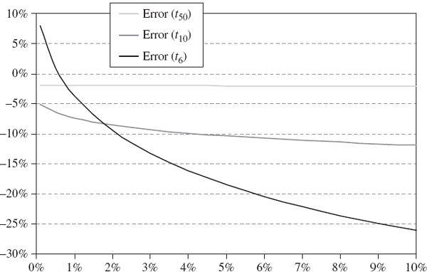
Figure IV.3.15 illustrates the error arising from a Cornish–Fisher VaR approximation when the underlying return distribution is known to be a Student t distribution. We consider three different degrees of freedom, i.e. 6, 10 and 50 degrees of freedom, to see how the leptokurtosis in the population influences the fit of the Cornish–Fisher approximation to the true quantiles. The horizontal axis is the significance level of the VaR – in other words, the quantile that we are estimating with the Cornish–Fisher approximation.

The Student t VaR is given by (IV.2.62). This is the ‘true’ VaR because, for a given value of the degrees of freedom parameter, the quantiles along the horizontal axis are exactly equal to the Student t quantiles. Then, for each quantile, the error is defined as the difference between the Cornish–Fisher VaR and the Student t VaR, divided by the Student t VaR.

Figure IV.3.15 Error from Cornish–Fisher VaR approximation

With 50 degrees of freedom the population has very small excess kurtosis (of 0.13) and the Cornish–Fisher approximation to the VaR is very close. In fact, the Cornish–Fisher approximation underestimates the true VaR by only about 2%. When the population has a Student t VaR with 10 degrees of freedom, which has an excess kurtosis of 1, Cornish–Fisher also underestimates the VaR, this time by approximately 10%. But the errors that arise when the underlying distribution is very leptokurtic are huge. For instance, under the Student t distribution with 6 degrees of freedom, which has an excess kurtosis of 3, the Cornish–Fisher VaR considerably underestimates the VaR, except at extremely high confidence levels. We conclude that the Cornish–Fisher approximation is quick and easy but it is only accurate if the portfolio returns are not too highly skewed or leptokurtic.

IV.3.4.4 Johnson Distributions

A random variable X has a Johnson SU distribution if

where Z is a standard normal variable and sinh is the hyperbolic sine function.³² The parameter ξ determines the location of the distribution, λ determines the scale, γ the skewness and δ the kurtosis. Having four parameters, this distribution is extremely flexible and is able to fit most empirical densities very well, provided they are leptokurtic.

It follows from (IV.3.9) that each α quantile of X is related to the corresponding standard normal quantile z_α = Φ⁻¹(α) as

Let X denote the h-day return on a portfolio. Then the 100α% h-day historical VaR of the portfolio, expressed as a percentage of the portfolio value, is − x_α.³³ Hence, under the Johnson SU distribution

Thus, if we can fit a Johnson SU curve then we can use (IV.3.11) to estimate the VaR.

It is possible to fit the parameters of the Johnson SU distribution, knowing only the first four moments of the portfolio returns, using a simple moment matching procedure. For the examples in this chapter, this moment matching procedure has been implemented in Excel using the following algorithm, developed by Tuenter (2001):

1. Set ω = exp(δ⁻²).
2. Set

   

   where is the sample excess kurtosis.

3. Calculate the upper bound for ω:

   

4. Calculate the lower bound for ω:

   

   where ω₁ is the unique positive root of ω⁴ + 2ω³ + 3ω² − −6 = 0, and ω₂ is the unique positive root of (ω − 1)(ω + 2)² = ², where is the sample skewness.

5. Find ω such that ω^lower< ω ≤ ω^upper and

   

6. Now the parameter estimates are:

   

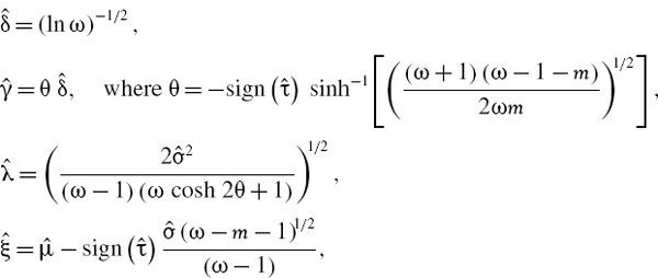
   where and are the mean and standard deviation of the portfolio returns.

Note that there are three numerical optimizations involved: first in steps 3 and 4 of the algorithm we use Goal Seek twice to find the upper and lower bound for ω, and then in step 5 we apply Solver.³⁴

EXAMPLE IV.3.5: JOHNSON SU VAR

Estimate the Johnson 1% 10-day VaR for a portfolio whose daily log returns are i.i.d. with skewness −0.2 and excess kurtosis 4, assuming that the mean excess return is 2% per annum and the portfolio's volatility is 25%.

SOLUTION Figure IV.3.16 illustrates the spreadsheet that is used to implement Tuenter's algorithm. Hence, we calculate the 1% 10-day VaR of the portfolio as 13.68% of the portfolio's value, using a Johnson SU distribution to fit the sample moments. This should be compared with 11.55% of the portfolio value, under the assumption that the portfolio returns are normally distributed.

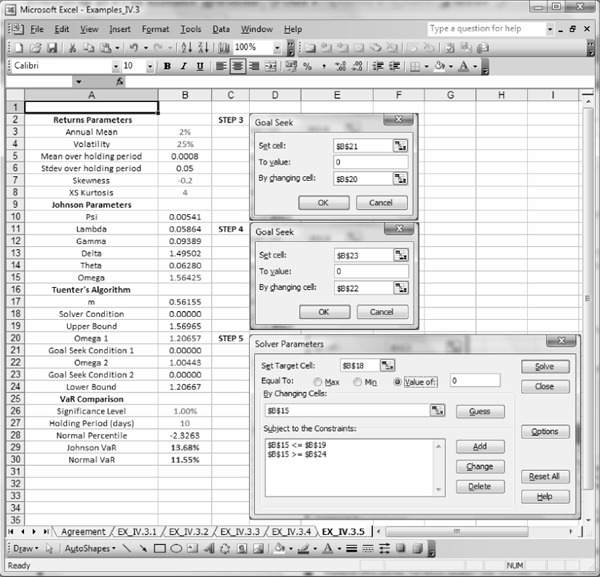
Figure IV.3.16 Tuenter's algorithm for Johnson VaR

We know from the previous subsection that Cornish–Fisher VaR is not a good approximation to VaR at extreme quantiles when the portfolio return distribution is very leptokurtic. Can Johnson's algorithm provide better approximations to the historical VaR at extreme quantiles than Cornish–Fisher VaR? Figure IV.3.17 demonstrates that the answer is most definitely yes. This figure shows the errors arising from the Johnson approximation to the same Student t populations as those used in Figure IV.3.15, and they are much lower than those arising from the Cornish–Fisher approximations in Figure IV.3.15.

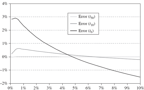
Figure IV.3.17 Error from Johnson VaR approximation

The error in the VaR estimate is virtually zero when the Johnson distribution is fitted to the Student t distribution with 50 degrees of freedom (excess kurtosis 0.13) and the error when it is fitted to the Student t VaR with 10 degrees of freedom is also negligible. Under the Student t distribution with 6 degrees of freedom (excess kurtosis 3), the Johnson VaR slightly underestimates the VaR at quantiles between 5% and 10% and slightly overestimates it at quantiles between 0.001% and 5%.

IV.3.5 HISTORICAL VALUE AT RISK FOR LINEAR PORTFOLIOS

Until now we have been focusing on the general features of historical VaR, and the ways in which the standard ‘vanilla’ historical simulation can be extended to improve the sample data (e.g. via volatility adjustment) and the accuracy of historical VaR at high levels of confidence. Throughout we have assumed that a risk factor mapping has already been applied to obtain a historical sample of returns for the portfolio. We shall now focus on the use of risk factor mapping in the context of historical VaR.

This section provides a sequence of five case studies that describe the estimation of historical VaR for different types of portfolio. We consider bonds, loans and swaps portfolios and any other interest rate sensitive portfolio that is represented by a sequence of cash flows, as well as stock and commodity portfolios. As in Chapter IV.2, we assume that readers are already familiar with the portfolio mapping methodologies for each type of portfolio.³⁵ Our main focus will be on the link between the asset class and the structure of the historical simulation model. For the sake of clarity, we shall not be as concerned with the precision of the estimate as we were in the previous section. We do not attempt to improve the accuracy of the VaR estimate by fitting a kernel or a parametric distribution, or by using Cornish–Fisher or Johnson approximations, and we shall only use the simple square-root-of-time scaling rule. However, in most of the case studies we shall examine the effects of a volatility adjustment. Even so, in order not to detract from our main focus, volatility adjustment is based on a simple EWMA model rather than a more sophisticated GARCH model.³⁶

We begin in Section IV.3.5.1 with a case study that demonstrates how historical simulation is applied to an interest rate sensitive portfolio that is represented as a sequence of cash flows. We compare the historical VaR estimate to that obtained using a parametric linear VaR model on the same data. The case study in Section IV.3.5.2 considers a simple domestic stock portfolio, estimating the historical VaR first without and then with a risk factor mapping. We explain how to decompose the total historical VaR into systematic VaR due the risk factors and the residual or specific VaR. The case study in Section IV.3.5.3 examines a large international portfolio of stocks and bonds, and explains the decomposition of total systematic VaR into equity, interest rate and forex stand-alone VaRs, and into the corresponding marginal VaRs, all in the historical VaR framework. Section IV.3.5.4 estimates the interest rate, forex and total historical VaR of an international bond position and the final case study in Section IV.3.5.5 is on the decomposition of historical VaR for an energy trader in crack spreads.

IV.3.5.1 Historical VaR for Cash Flows

This case study uses historical simulation to estimate the VaR of the UK bond portfolio that was the subject of the case study in Section IV.2.4. As before, we assume that the cash flows on the portfolio have been mapped to a set of standard maturity interest rates, which are the UK spot interest rates at monthly maturities up to 5 years. So these are the portfolio's risk factors. The portfolio's PV01 vector on 31 December 2007 was depicted in Figure IV.2.2.

In this case study we shall estimate the historical VaR of the same portfolio, but now we need a very large sample of data on the risk factors. We shall use daily data starting on 4 January 2000 and ending at the time the VaR is estimated, i.e. on 31 December 2007. Thus we have 8 years of data on the interest rate risk factors, and these are illustrated in Figure IV.3.18. From the figure it is clear that UK interest rates passed through several different regimes during the sample period.

To find the historical VaR we must map the portfolio to its risk factors. Thus a historical series of daily P&L on the portfolio is constructed by holding the PV01 vector of the portfolio constant.³⁷ We apply this to each of the daily returns over the sample period using the risk factor mapping

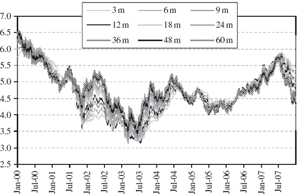
Figure IV.3.18 Bank of England short curve

which we already know may also be written in matrix form as

where p =(PV01₁, PV01₂,…, PV01₆₀)′ is the PV01 vector and Δr_t = (ΔR_1t, ΔR_2t,…,ΔR_60t) is the vector of daily interest rate changes at time t. The 100α% 1-day historical VaR is minus the α quantile of the P&L distribution. For longer holding periods the historical VaR is obtained using a square-root scaling rule.³⁸

Such a large sample of daily data will allow the historical VaR to be estimated at fairly high confidence levels with reasonable accuracy. But if a long historical sample is used, we know from our discussions in Section IV.3.3.3 that a volatility adjustment should be applied to the daily changes in interest rates before estimating the VaR. A simple EWMA volatility estimate will be used, and the quickest and most effective way to do this is not on the risk factors, but on the P&L of the portfolio. The EWMA volatility of the portfolio's P&L is shown in Figure IV.3.19.³⁹

First suppose that we are estimating VaR at the end of the sample, i.e. on 31 December 2007. At this time UK interest rate volatility was greater than it had been since January 2004, so a volatility adjustment will increase the dispersion of the return distribution. Figure IV.3.20 depicts the portfolio's daily P&L distribution, before and after the volatility adjustment, based on the entire sample.

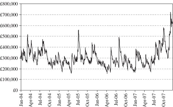
Figure IV.3.19 EWMA volatility of P&L on UK gilts portfolio

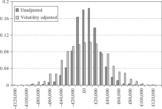
Figure IV.3.20 Empirical distribution of UK gilts portfolio P&L on 31 December 2007

The excess kurtosis in the unadjusted P&L is huge – it is approximately 45 – but after volatility adjustment this is very significantly decreased. In fact, after volatility adjustment the excess kurtosis over the entire sample is −0.2267, so the adjusted P&L distribution is very slightly mesokurtic rather than leptokurtic. The volatility adjustment increases the small positive skewness from approximately 0.03 to approximately 0.07. Since negative excess kurtosis and positive skewness both serve to reduce the VaR relative to the normal VaR, after volatility adjustment we expect the historical VaR based on the entire sample to be very slightly less than the normal VaR.

Table IV.3.12 reports the 10-day historical VaR for the portfolio, with and without volatility adjustment, at the 1% and the 0.5% significance levels.⁴⁰ This is compared with the corresponding normal VaR, again with and without volatility adjustment.⁴¹

Table IV.3.12 Historical versus normal VaR for UK bond portfolio

Table IV.3.12 is based on the entire sample from 5 January 2000 to 31 December 2007. But in the spreadsheet for this case study the reader may change the sample used to estimate the VaRs, including the time at which the VaR is measured, and by changing the PV01 vector the reader can also change the portfolio.

IV.3.5.2 Total, Systematic and Specific VaR of a Stock Portfolio

The case study in this section considers the historical VaR for a simple portfolio consisting of two stocks in the S&P 100 index, Apple Inc. and Citigroup Inc.⁴² First we measure the total VaR using a long historical series of portfolio returns, based on a constant portfolio weights assumption. Then we decompose the total VaR into a systematic VaR component, due to movements in the S&P 100 index, and a specific VaR component, due to the idiosyncratic movements of each stock price.

The total historical VaR of an equity portfolio is calculated from a distribution of ‘reconstructed’ portfolio returns, in this case where the portfolio weights are held constant at their current values. Denote the date on which the VaR is calculated by T and the date of each set of returns on the stocks by t, for t = 1,…, T. On each date t in the historical sample the portfolio return is calculated as

where w_T is the portfolio weights vector at time T (when the VaR is measured) and x_t is the vector of stock returns at time t.

Since the historical VaR will better reflect current market conditions when volatility adjusted stock returns are used, the next example compares the historical VaR estimates with and without volatility adjustment. However, the volatility adjustment may be computed in two different ways:

(i) adjust the volatility of each stock return and then apply the portfolio weights, or

(ii) apply the weights to obtain the portfolio returns r_t and then volatility-adjust these returns.

The complication with (i) is that an individual volatility adjustment of each stock return would change their correlation, unless we apply the volatility adjustment in the context of a multivariate system. For this, following Duffie and Pan (1997) we use the Cholesky matrix of the covariance matrix of stock returns, in place of the square root of the variance of each stock return, in the volatility adjustment (IV.3.3).

To be more specific, suppose there are k stock returns and a total of T observations on each return in the historical sample. Denote the GARCH (or EWMA) covariance matrix of the stock returns at time t by V_t and denote the Cholesky matrix of V_t by Q_t. In other words,

Now set

Then

Thus _t is a vector of stock returns at time t that is adjusted to have the constant covariance matrix V_T, for all t = 1,…, T.

The following example demonstrates the differences that will arise, depending on the method of volatility adjustment.⁴³ As in the previous subsection, so as not to make the illustration too complex, instead of using a GARCH model we shall use a simple EWMA volatility adjustment for the daily VaR, with square-root scaling over a 10-day risk horizon.

EXAMPLE IV.3.6: VOLATILITY-ADJUSTING HISTORICAL VAR FOR A STOCK PORTFOLIO

You hold a portfolio on 21 April 2007 that has 30% invested in Citigroup Inc. stock and 70% invested in Apple Inc. stock. Assuming the returns are i.i.d., use daily returns data from 2 January 2001 to 21 April 2008 on the closing prices of these stocks to estimate the 100α% 10-day historical VaR, for α = 0.001, 0.01, 0.05 and 0.1 and compare the results obtained before and after volatility adjustment.

SOLUTION The evolution of the prices of the two stocks over the sample period is shown in Figure IV.3.21. The Citigroup price is on the left-hand scale and the Apple price is on the right-hand scale. Figure IV.3.22 shows the EWMA volatilities of each stock over the sample period. For the volatility adjustment in this case study we shall employ the same value for the smoothing constant in all the EWMA models that are applied, for both the estimation of portfolio betas and volatility adjustment of returns series. This is an ad hoc choice, so let us fix λ at the RiskMetrics™ value of 0.94.⁴⁴ Whilst both stock price volatilities displayed significant time variation over the sample period, and their volatility in April 2008 is high, both stocks also had high volatilities in the early part of the sample. Hence, it is unclear whether volatility adjustment would reduce or increase the historical VaR estimates.

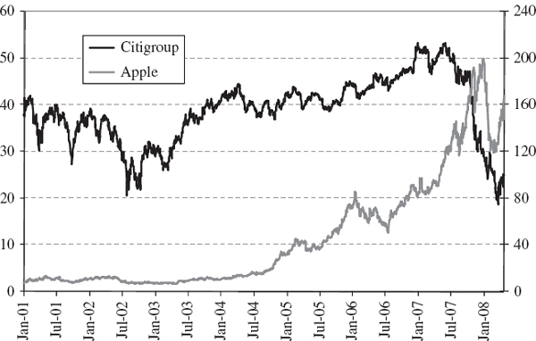
Figure IV.3.21 Apple and Citigroup stock prices

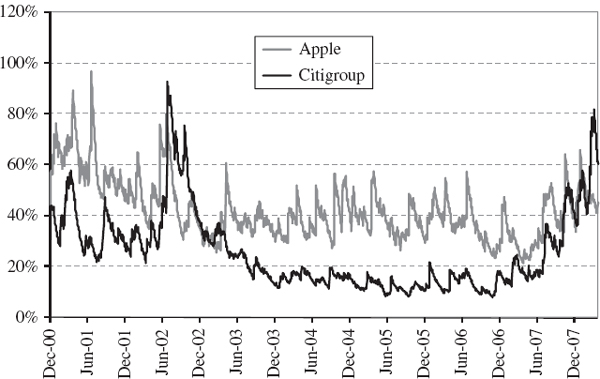
Figure IV.3.22 EWMA volatilities of Apple and Citigroup

The unadjusted historical VaR is calculated using the Excel PERCENTILE function on the portfolio returns series (IV.3.14), where w_T =(0.3, 0.7)′ and the returns vector x_t is a 2 × 1 vector of the unadjusted daily returns on Citigroup and Apple stocks at time t. We shall consider three ways to obtain the volatility adjusted portfolio returns:

(a) Estimate the EWMA covariance matrix of the two stock returns. Then we can adjust each of the stock returns to have constant volatility using (IV.3.15), and then we compute (IV.3.14) using the adjusted returns for x_t.

(b) Compute the portfolio's returns in the usual way, then adjust these to have constant volatility using (IV.3.3).

(c) Ignore the effect that volatility adjustment has on correlation and simply adjust each stock return to have constant volatility using (IV.3.3), and then compute (IV.3.14) using the volatility adjusted returns for x_t.

Does the VaR change much, depending on the method used? Table IV.3.13 reports the results.

Table IV.3.13 Historical VaR with different volatility adjustments

Clearly, some form of volatility adjustment is important. At low confidence levels (e.g. 90%) the unadjusted VaR is lower than the adjusted VaRs, and the opposite is the case for very high confidence levels (e.g. 99.9%). This implies that without the adjustment the historical return distribution is much more leptokurtic. But the method used to perform the volatility adjustment makes only a small difference to the result. At every confidence level the greatest VaR is obtained using method (a) and the lowest VaR is obtained using method (c), but the results are similar.

Should we adjust the stock returns before computing the portfolio's returns or adjust the portfolio returns? The answer depends on computation time, if this is a constraint. For instance, if we need to measure the VaR for many different portfolios in the same stock universe (or sharing the same risk factors) it may be more efficient to adjust each returns series before the portfolios returns are formed, and the correct method to use is (a). That is, we should use the entire covariance matrix to adjust the returns, rather than just the volatility of each return separately. However, method (c) is quicker and easier than (a) and, although it is approximate, the error it introduces is not large relative to the huge model risk that plagues many VaR models.

When a portfolio is mapped to its risk factors we can decompose the total VaR of the portfolio into the systematic VaR, due to changes in the risk factors, and the specific VaR which is not captured by the risk factor mapping. We have done this before in the context of normal linear VaR. In that model the square of the total VaR is equal to the sum of the square of the systematic VaR plus the square of the specific VaR. Unfortunately, there are no such simple aggregation rules between total VaR, systematic VaR and specific VaR in either the historical simulation or the Monte Carlo simulation VaR frameworks. Nevertheless we may still decompose total VaR into systematic and specific components.

We aim to estimate the systematic and specific VaR of the Apple and Citigroup portfolio, and to do this we must first estimate the portfolio betas with respect to an index; we choose the S&P 100 index for illustration.⁴⁵ To ensure that these are as risk sensitive as possible, we estimate the betas using EWMA instead of ordinary least squares regression. This method was described in full when we first introduced factor models for equity portfolios in Section II.1.2 and in Section II.3.8, so we merely provide a spreadsheet in the case study that illustrates the estimation of these betas, allowing the reader to change the smoothing constant. The S&P 100 betas corresponding to λ = 0.94 are shown in Figure IV.3.23.

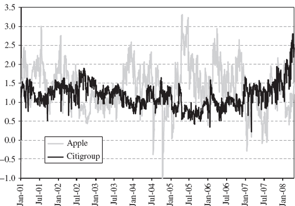
Figure IV.3.23 EWMA betas for Apple and Citigroup in S&P 100 index

The EWMA beta estimate varies over the sample period but it is only the current estimate of the beta (i.e. the estimate in the last sample period, at time T) that is used to construct the portfolio's systematic returns. With a smoothing constant of 0.94, we obtain

where the first element is the beta for Apple and the second is for Citigroup.⁴⁶ Notice that the beta of Citigroup rose considerably during the credit crisis at the end of the period. The Citigroup beta was lower and less variable than the Apple beta in the earlier part of the sample, but since the credit crunch in 2007 it has become the more risky of the two stocks.

Fixing the stock betas at their current values, we now compute the systematic part of the portfolio return _t using

where w_T represents the weights and β_T is the beta vector at time T when the VaR is measured, and M_t is the index return at time t. In the next example we use the weights w_T =(0.3, 0.7) as before, the market index is the S&P 100 and the betas are given by (IV.3.16).

EXAMPLE IV.3.7: SYSTEMATIC AND SPECIFIC COMPONENTS OF HISTORICAL VAR

As in Example IV.3.6, suppose you hold a portfolio that has 30% invested in Citigroup Inc. stock and 70% invested in Apple Inc. stock. Using the S&P 100 index as the risk factor, decompose the total 1% 10-day VaR of your portfolio, with and without a EWMA volatility adjustment, into systematic and specific components. Estimate the VaR on 21 April 2008 and compare your results with the VaR that is estimated on 30 October 2006 for the same portfolio, i.e. with 30% invested in Citigroup and 70% invested in Apple. In each case, use data starting on 2 January 2001 and express the VaR as a percentage of the portfolio value.

SOLUTION We know from the previous example that our estimate of the total VaR of the portfolio depends on whether we apply volatility adjustment and, if so, how this is performed. The portfolio's systematic returns are obtained using (IV.3.17). Figure IV.3.24 shows the results before and after volatility adjustment. Figure IV.3.24(a) shows the returns adjusted for the relatively low volatility on 30 October 2006, and Figure IV.3.24(b) shows the returns adjusted for the relatively high volatility on 21 April 2008.

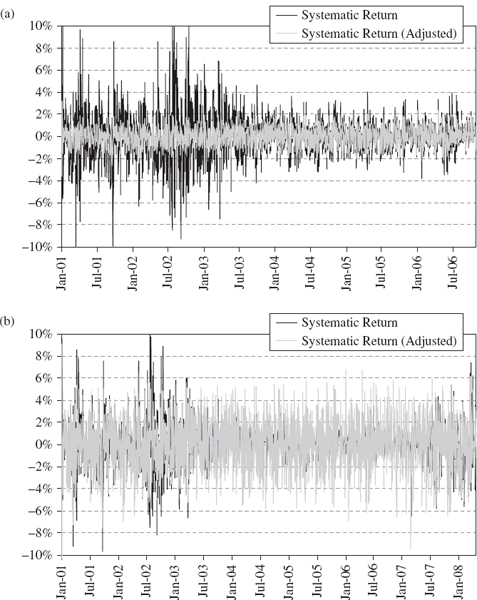
Figure IV.3.24 Systematic returns before and after volatility adjustment for the volatility on (a) 30 October 2006 and (b) 21 April 2008

The specific returns, which are the portfolio returns minus the systematic returns, are also adjusted for volatility. Finally, we calculate the 1% 10-day historical VaR from the relevant quantile of each distribution, obtaining the results shown in Table IV.3.14. For comparison, we also include the normal linear VaR based on the same data. Results for other portfolio weights, data periods, significance levels and risk horizons can be generated by changing the dates and parameters in the spreadsheet for this example in the case study workbook.

Table IV.3.14 Total, systematic and specific VaR, US stock portfolio

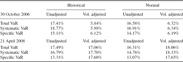
On 30 October 2006 the 1% 10-day total VaR of the portfolio was 17.41% of the portfolio value before volatility adjustment but only 5.84% after adjusting for the low volatility leading up to this time. As Figure IV.3.24(a) shows, the extreme volatility of the portfolio during 2001–2003 means that the historical VaR will be much larger before the volatility adjustment. The systematic VaR is greater than the total VaR of the portfolio, and even the specific VaR is greater than the total VaR after the volatility adjustment.⁴⁷ It is again evident that the volatility adjustment decreases the excess kurtosis of the returns to such an extent that it becomes negative. We can see this from the fact that the normal linear VaR estimates are greater than the historical VaR estimates after the volatility adjustment, but not before.

A different picture emerges on 21 April 2008 (for which the systematic returns are shown in Figure IV.3.24(b)). The volatility at the time the VaR is measured was less than it was during 2001–2003 but higher than it was during 2004–2006, and so the volatility adjustment makes little difference to the VaR estimate based on the period 2001–2008. Still, the volatility adjustment alters the shape of the empirical distribution, slightly increasing the volatility but also decreasing the excess kurtosis. Thus the normal VaR estimates still increase after the volatility adjustment, and the historical systematic VaR, and the specific VaR again become greater than the total VaR after the volatility adjustment.

IV.3.5.3 Equity and Forex VaR of an International Stock Portfolio

Because historical VaR is calculated as a quantile it does not obey simple aggregation rules, such as the sub-additivity rule that applies to parametric linear VaR, whereby total linear VaR is never greater than the sum of the stand-alone linear VaRs. Normal and Student t VaR obeys the same rules as the variance operator, but historical VaR obeys the same rules as quantiles, and quantiles obey very few rules.

Quantiles translate under continuous monotonic increasing transformations. That is, if the variable X has α quantile x_α then, for any continuous monotonic increasing function f, f(X) has α quantile f(x_α).⁴⁸ We call this the monotonic property of quantiles. Time aggregation of quantiles is also possible, but only under the assumption that portfolio returns are stable.⁴⁹

However, aggregation of historical VaR across positions is not the same as monotonic transformation or time aggregation. No aggregation rules such as sub-additivity apply, but this does not imply that we cannot decompose and aggregate historical VaR. Indeed, dependencies between returns play a very important role in reducing risk via diversification, and an attractive feature of the historical model is that we do not capture any dependency using a correlation matrix; instead the dependencies are implicit in the historical data.

We now present a case study to illustrate the disaggregation of total systematic VaR into stand-alone and marginal VaR components, when the VaR model is based on historical simulation. Consider a UK investor holding a US and a UK stock portfolio on 21 April 2008. Suppose 70% of the total amount invested in pounds sterling is held in UK stocks and 30% is held in US stocks. The US portfolio has a beta of 1.8 relative to the S&P 500 index and the UK portfolio has a beta of 1.25 relative to the FTSE 100 index.

To assess the historical VaR for this portfolio we use daily log returns on the S&P 500 index, the FTSE 100 index and the £/$ exchange rate from 3 January 1996 to 21 April 2008.⁵⁰ The indices themselves are shown in Figure IV.3.25, with the S&P 500 measured on the right-hand scale and the FTSE 100 measured on the left-hand scale. The £/$ forex rate is shown in Figure IV.3.26. This illustrates the fairly steady decline in the US dollar from January 2001 until the end of the sample. Hence, anything the investor has gained from his exposure to US stocks will be offset by losses on the currency position.

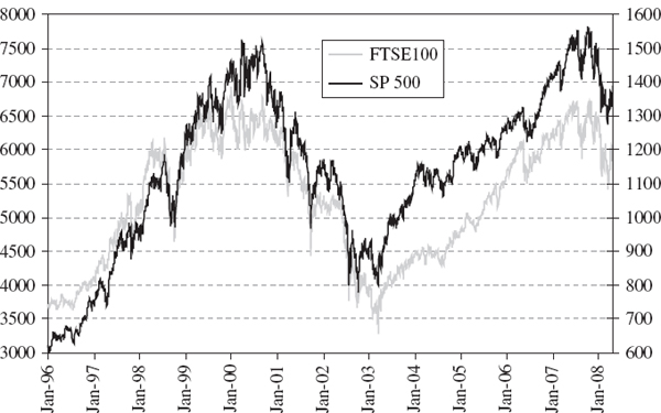
Figure IV.3.25 S&P 500 and FTSE 100 indices, 1996–2008

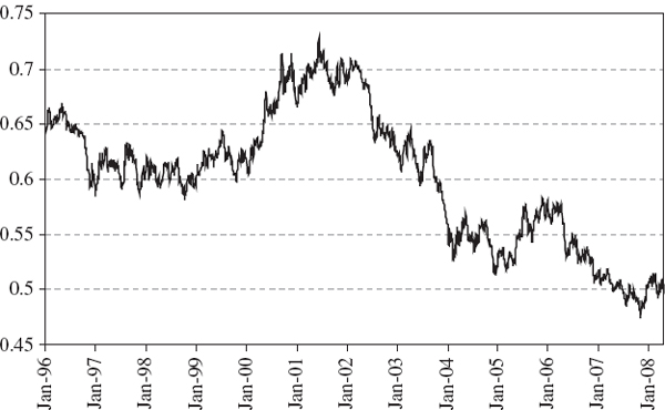
Figure IV.3.26 £/$ forex rate, 1996–2008

The VaR will be measured at an interesting time in equity markets. After several years of very low volatility stock markets in the US and the UK, volatility had risen following concerns about the Chinese and US economies and then in the aftermath of the sub-prime mortgage crisis, whose effects were still impacting stocks in the financial sector in April 2008. Since we use the entire sample with over 3000 observations, we shall estimate volatility adjusted historical VaR.⁵¹ Based on EWMA with λ = 0.94, the volatilities of the FTSE 100 and S&P 500 index and of the forex rate are depicted in Figure IV.3.27. By the end of the sample equity volatilities had climbed to around 25%, but the £/$ exchange rate remained stable with a volatility of approximately 10%.

We now explain the methodology that underpins the VaR disaggregation into equity and forex components. The price in pounds sterling is the dollar price multiplied by the £/$ exchange rate; or, in symbols, . Hence, the log equity return and the log forex return are additive. In other words, the log return on the US stock portfolio in pounds sterling is the sum of the log return on the US stock portfolio in US dollars and the log return on the £/$ rate:

Or, in alternative notation, . Hence, the risk of a US stock portfolio to a UK investor has an equity component, which is based on the risk of the dollar returns on the portfolio, and a forex component, which is based on the risk of the £/$ forex rate.

Figure IV.3.27 Volatilities of UK and US stock markets and the £/$ exchange rate

We have 70% of our capital invested in the UK portfolio, with sterling price at time t denoted by , and 30% of our capital is invested in the US portfolio, with sterling price . In other words, the total portfolio has a sterling price

where ω₁ = 0.7 and ω₂ = 0.3. From (IV.3.18) is follows that now it is the percentage return, not the log return, that is additive. This means that to disaggregate the total VaR into equity and forex components we must assume the percentage return is approximately equal to the log return. We know from Section I.1.4 that this approximation is accurate only when the return is small, and this is another reason why it is standard to base historical VaR estimation on high frequency (e.g. daily) data.

Let β₁ denote the percentage beta of the UK portfolio with respect to the FTSE 100 at the time the VaR is measured and let ω₁ denote the proportion of total capital invested in the UK portfolio. Similarly, let β₂ denote the percentage beta of the US portfolio with respect to the S&P 500 at the time the VaR is measured and let ω₂ denote the proportion of total capital invested in the portfolio US. Thus ω₁ + ω₂ = 1. In local currency, the daily log returns on the UK and US portfolios are denoted by and , and the daily log returns on the two equity indices are written and , so for i = 1, 2 and * = £ or $. The £/$ forex log return is denoted by as before.

Now, applying the log return approximation to the percentage return, we may write the sterling return on our combined portfolio of US and UK stocks as

On the right-hand side above we have two components to the portfolio return:

1. the net equity return,
2. the forex return, .

The return on the total portfolio is the sum of these.

Using historical data for each of the series of log returns (i.e. on the FTSE 100 index, the S&P 500 index and the £/$ exchange rate) we find the equity VaR and forex VaR from the quantiles of the corresponding empirical return distributions. Each time series runs from January 1996 until 21 April 2008. Adding the net equity return and forex return time series together gives a time series for the net portfolio return, and the total risk factor VaR is obtained from the quantile of this empirical distribution.

Table IV.3.15 presents the 100α% h-day risk factor VaR, disaggregated into equity and forex components. It is expressed as a percentage of the total sterling value of the US and UK portfolios and it is based on the entire sample of over 3000 observations.⁵² The forex stand-alone VaR is relatively small and the total VaR is only slightly more than the equity stand-alone VaR. Total risk factor VaR is less than the sum of the equity VaR and the forex VaR, although this need not always be the case with historical VaR, since it is measured as a quantile rather than a volatility. Since the portfolio's volatility has previously been both higher and lower than the volatility at the time the VaR is measured, the volatility adjustment makes little difference to the VaR. However, by changing the start and end dates in the spreadsheet, readers can see that this is not always the case.

Table IV.3.15 Decomposition of systematic VaR into equity and forex stand-alone components

We know from Section IV.1.7.3 that we measure the marginal VaR by estimating the gradient vector g (θ) of first partial derivatives of VaR with respect to the risk factor sensitivities. In the parametric linear VaR framework there are analytic formulae that can be applied to obtain the gradient vector, as for instance in Section IV.2.2.5. But in the historical VaR model there are no such analytical formulae. So we estimate g (θ) using a first order finite difference, as explained in Section I.5.5. That is, we make a small perturbation in each of the risk factor sensitivities in turn, and compute the first partial derivative of the total VaR with respect to that sensitivity by dividing the resulting change in the total VaR by the small perturbation.⁵³ The risk factor sensitivities, in percentage terms, are θ =(1, ω₂)′ on the equity and forex returns respectively.

Having estimated the gradient vector, we multiply each component in the vector by its risk factor sensitivity, before perturbation, to obtain the corresponding marginal VaR. For the portfolio in this case study the results are displayed in Table IV.3.16. Based on the unadjusted returns data from January 1996 to 21 April 2008, 92.29% of the total risk factor 1% 10-day VaR is due to equity risk and only 7.71% is due to forex risk. At the 0.1% significance level a slightly greater percentage of the VaR is due to equity risk. Note that when based on the volatility adjusted returns (which we know usually have less kurtosis than unadjusted returns) the contribution of forex risk to the total VaR is much smaller, and it can even be negative.

Table IV.3.16 Historical marginal VaR for international stock portfolio

IV.3.5.4 Interest Rate and Forex VaR of an International Bond Position

We now consider a case study where a UK bank buys £50 million nominal of an AA-rated 5-year US bond with an annual coupon of 4% on 21 April 2008. Since the bank needs to purchase £50 million in US dollars to finance the purchase, the total return will also have a currency component. So the risk factors are the US swap curve, which is AA-rated, and the sterling–dollar exchange rate. We shall decompose the historical VaR into interest rate and forex components.

Daily historical data on US swap rates from July 2000 until 21 April 2008 are shown in Figure IV.3.28.⁵⁴ The swap curve is upward sloping, except for two relatively flat periods during 2001 and during 2006–2007, and short term rates varied more than longer terms rates over the sample. The highest value for the 1-year swap rate was 7% at the beginning of the sample and its lowest value was about 1%, in June 2006.

The interest rate VaR is based on a P&L distribution that can be estimated in two approximately equivalent ways, either using the PV01 approximation to the bond P&L given by (IV.3.12) or by revaluing the bond directly. For the first approach the PV01 vector for the bond is calculated in the spreadsheet labelled VaR, using the approximation described in Section IV.2.3.2, and this is the PV01 vector reported in the last row of Table IV.3.17. This table also shows the price P of the bond per £100 nominal, and the number of units of £100 nominal that the bank purchases for £50 million cash, which is given by N = 50 × 10⁶ × P⁻¹. Holding this PV01 vector constant, we apply (IV.3.12) with the historically observed time series of basis point changes to swap rates. This gives a time series of P&L on the bond that is shown in column H of the spreadsheet labelled ‘VaR’ in the case study workbook.

Figure IV.3.28 US swap rates

Table IV.3.17 Bond position

Another way to derive a historical P&L distribution for a bond position is to apply the historical daily basis point changes to the current swap curve, and then to revalue our cash position keeping N constant. This gives the values in column I of the spreadsheet labelled VaR. Then the historical P&L is obtained by taking each simulated value and deducting the current value of £50 million. These P&L are shown in column J of the same spreadsheet. Note that the two approaches give almost identical results.⁵⁵

The total VaR is based on the US dollar P&L distribution, and the dollar price at any point in time is the price in pounds multiplied by the $/£ exchange rate. The forex VaR is estimated from the historical distribution of daily log returns on the $/£ exchange rate, and the P&L distribution for the total VaR is obtained by converting the position value in column I into US dollars, and then recalculating the P&L. To find the relevant exchange rate to apply for each day, we apply the log return on the forex on that day to the current forex rate, i.e. the rate at the time the VaR is measured. The resulting P&L is shown in column L.

In each case the VaR is minus the α quantile of the daily P&L distribution, and the 1-day VaR estimates are multiplied by the square root of the risk horizon (in days) to estimate the corresponding h-day VaR.⁵⁶ The results for 1% 10-day VaR are given in the spreadsheet in both pounds sterling and US dollars, and the sterling figures are displayed in Table IV.3.18.

Table IV.3.18 VaR decomposition for international bond position

Interest Rate VaR (PV01 approx.)	£1,381,833
Interest Rate VaR (direct valuation)	£1,374,072
Forex VaR	£2,319,324
Total VaR	£2,042,953

As already mentioned, it makes very little difference whether we estimate the interest rate VaR using the PV01 approximation or the bond evaluation method. The forex VaR is greater than the interest rate VaR, and the total VaR is less than the square root of the sum of the squared component VaRs, which indicates a small or negative dependency between the £/$ rate and the swap rates.

IV.3.5.5 Case Study: Historical VaR for a Crack Spread Trader

In this subsection we consider a trader in crack spread futures. There are two crack spreads, i.e. the difference between the heating oil futures price and the WTI crude oil futures price of the same maturity, and the difference between the gasoline futures price and the WTI crude oil futures price of the same maturity. NYMEX facilitates crack spread trading in its futures markets by treating both legs of the trade as a single transaction. Each futures contract is for 1000 barrels, priced in US dollars per barrel.

Because spreads can have negative values, it makes no sense to compute percentage returns on these risk factors, for the reasons explained in Section 1.5.5. Instead we compute the daily P&L on the crack spread futures and compute the VaR directly in nominal terms. We shall calculate the historical VaR of the entire portfolio, and then decompose the total VaR into the VaR due to the heating oil crack spread and the VaR due to the unleaded gasoline crack spread.

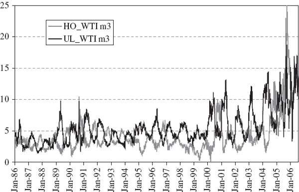
Figure IV.3.29 Three-month crack spread futures prices

Our risk factors are constant maturity futures on each spread for 1, 2, 3, 4, 5 and 6 months ahead.⁵⁷ The case study workbook contains over 20 years of daily data on these constant maturity futures, and the reader may use the spreadsheet labelled ‘VaR’ in this workbook to estimate the historical VaR, with and without volatility adjustment, using any start and end dates during this sample. The 3-month crack spread futures prices from 2 January 1996 to 1 August 2006, the day when the VaR is estimated, are shown in Figure IV.3.29. The trader's positions in crack spread futures, and their prices on 1 August 2006, are shown in Table IV.3.19.⁵⁸

Table IV.3.19 Crack spread book, 1 August 2006

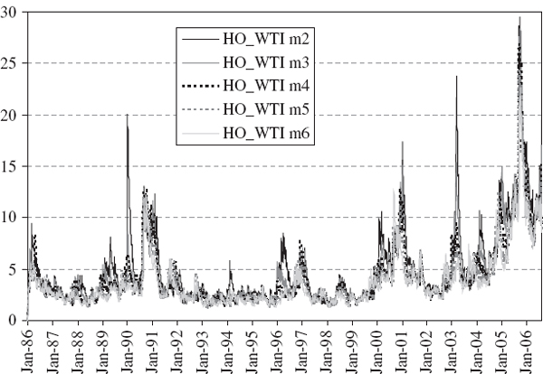
Figure IV.3.30 EWMA volatilities of heating oil crack spread futures P&L

Figures IV.3.30 and IV.3.31 show the volatilities of the crack spread futures P&L, calculated as an exponentially weighted moving average of squared daily changes in the futures price with a smoothing constant of 0.94.⁵⁹ These graphs display terrific variability in spread futures volatilities, so it is advisable to apply a volatility adjustment to the portfolio's P&L, and we shall use the EWMA volatilities shown in Figures IV.3.30 and IV.3.31 to derive a simple volatility adjustment, as described in Section IV.3.3.3. Since volatility was relatively high on 1 August 2006, the volatility adjusted VaR on 1 August 2006 is likely to be much greater than the VaR based on unadjusted P&L.

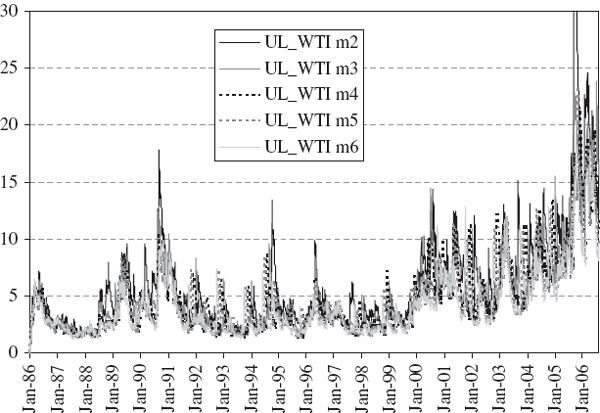
Figure IV.3.31 EWMA volatilities of gasoline crack spread futures P&L

In the case study workbook we hold the positions constant, at their values shown in Table IV.3.19, and simulate a historical series for the P&L on each futures position. The P&L series is simulated by multiplying the fixed number of contracts by the absolute change in the value of the spread on each day in the historical sample, after the volatility adjustment if this is used. Then we sum the P&L on each day due to (a) the six positions on heating oil crack spread futures of different maturities, and (b) the six positions on unleaded gasoline crack spread futures of different maturities, and (c) the 12 positions over all the futures. This gives three historical P&L series: one for the heating oil crack spread positions, another for the gasoline crack spread positions, and a third for the total positions. The historical VaR is calculated by finding the quantile of the simulated P&L distribution and then multiplying this quantile by −1000, since each futures contract is for 1000 barrels.

The reader may change the positions, the VaR parameters and the period over which the VaR is estimated in the spreadsheet labelled ‘VaR’. The 1% 10-day VaR results for the positions in Table IV.3.19, with and without volatility adjustment, are given in Table IV.3.20. The volatility adjustment increases the VaR very considerably, since the spreads were unusually volatile at the time when the VaR is measured. The total VaR is much less than the sum of the two stand-alone VaRs, but still greater than the square root of the sum of the squared stand-alone VaRs, because there is a high positive correlation between the spreads.

Table IV.3.20 Total VaR and component VaRs for a crack spread trader

IV.3.6 ESTIMATING EXPECTED TAIL LOSS IN THE HISTORICAL VALUE-AT-RISK MODEL

Section IV.2.11 derived analytic formulae for expected tail loss in parametric linear VaR models. This was possible because the model makes an assumption about the functional form of the return distribution. In the historical VaR model the ETL must be estimated directly, simply by taking the average of all the losses in the tail below the VaR. The exception is when a parametric distribution or approximation has been fitted to the historical distribution. In this case it is sometimes possible to derive an analytic formula for ETL.

In this section we first present some analytic formulae for the ETL when the historical distribution is fitted with a generalized Pareto distribution, a Johnson SU distribution and when the VaR is estimated using a Cornish–Fisher expansion. We end with a case study that compares the historical ETL estimates that are derived using these formulae with the historical ETL that is estimated directly, as the average of the losses that exceed the VaR.

IV.3.6.1 Parametric Historical ETL

From formula (I.3.68) derived in Section I.3.3.10 for the mean excess loss in the generalized Pareto distribution, it immediately follows that

where the parameters β and ξ are estimated by fitting a GPD to excess losses and VaR_α is given by (IV.3.6).

The other two ETL formulae are derived from the transformation of the random variable into a standard normal variable. Using the fact that the standard normal 100α% ETL is α⁻¹(Z_α),⁶⁰ for a Johnson SU distribution we have

Finally, it follows from (IV.3.7) that the ETL under the Cornish–Fisher expansion is approximated by

where

IV.3.6.2 Empirical Results on Historical ETL

We now present a case study that compares several estimates of the historical ETL. Using volatility adjusted log returns on the S&P 500 from 4 January 1950 until 9 March 2007, a GPD has been fitted to the excess returns over a threshold u, and the Cornish–Fisher expansion and the Johnson SU distribution have been fitted to the first four moments of the empirical returns. We compare the results from applying (IV.3.20)– (IV.3.22) with the results from the empirical ETL, estimated as the average of the losses in excess of the VaR, and with the ETL under the assumption that the returns are normally distributed.

There are over 14,000 returns in the sample, which allows for a comparison of results at very high significance levels. Of course the Cornish–Fisher and Johnson ETL can be estimated from a very much smaller sample, because they require only the first four moments of the empirical return distribution. However, the GPD requires a considerable amount of data, since it is fitted only to the excess losses over a certain threshold.

We set significance levels 1%, 0.1% and 0.05%, corresponding to confidence levels of 99%, 99.9% and 99.95% respectively, and the results from estimating the daily VaR using the different models are displayed in Table IV.3.21. As usual the VaR estimates are reported as a percentage of the portfolio value at the time the VaR is estimated. The Johnson VaR estimates are generally closer to the GPD estimates but they do not suffer the disadvantage of the GPD VaR estimates, i.e. that they are sensitive to the choice of threshold. Moreover, as described in Section IV.3.4.4, estimation of Johnson SU parameters is straightforward, using the algorithm developed by Tuenter (2001). This algorithm is implemented in the spreadsheet for this case study.

Table IV.3.21 Estimates of GPD parameters and historical VaR estimates

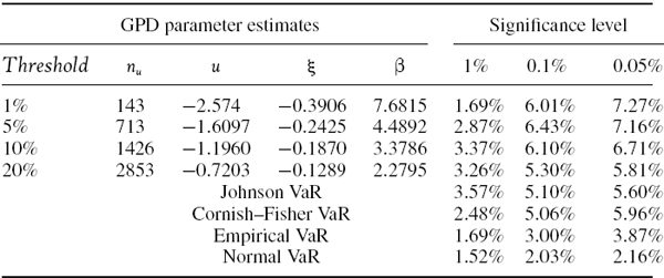
Table IV.3.22 compares the daily historical ETL estimates based on a normal approximation to the return distribution, the empirical distribution. Notice that those based on the GPD, Johnson and Cornish–Fisher parametric fits. The empirical returns have an excess kurtosis of 4.93 and a very significant negative skewness. As a result the normal ETL estimates are far too low, and all the non-normal parametric ETL estimates exceed the empirical ETL. Even when the empirical ETL is based on 14,000 returns, the 0.1% ETL estimates are based on only 14 observations and the 0.05% ETL estimates are based on only 7 observations. Hence, they are likely to be imprecise.

Tables IV.3.21 and IV.3.22 indicate that there is a considerable degree of model risk associated with estimating VaR and ETL using historical simulation. There are very significant differences between the results that are obtained using different enhancements to the simulation model, particularly at very high confidence levels. So what advice, if any, can we glean from these diverse results?

Table IV.3.22 Comparison of ETL from parametric fits to historical return distribution

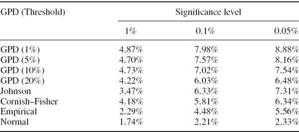
It is unlikely that risk analysts will be working with a sample having more than a few thousand observations, and the smaller the sample, the greater the model risk arising from the choice of parametric or semi-parametric method that is used to estimate the VaR and ETL. If the analyst does have a very large sample and therefore considers the use of the GPD, it seems better to use a relatively high threshold such as 20%, so that the tail contains a larger sample of returns.

IV.3.6.3 Disaggregation of Historical ETL

Historical ETL can be aggregated and disaggregated just like historical VaR, so we may compute stand-alone ETLs corresponding to different sub-portfolios. But, unlike historical VaR, the ETLs are always sub-additive. We now illustrate the disaggregation methodology with an extension of the case study in Section IV.3.5.3, where we disaggregated the total systematic VaR for an international equity portfolio consisting of US and UK stocks into equity and forex stand-alone components. In this case study we estimate the 100α% h-day historical ETL for the same portfolio.

The results for the 1% 10-day historical VaR and ETL estimated on 21 April 2008, using the same data as in Section IV.3.5.3, are displayed in Table IV.3.23. The upper part of the table shows the 1% 10-day historical VaR based on both unadjusted and EWMA volatility adjusted returns. These are identical to those reported in Table IV.3.15 for a significance level of 1% and h = 10. The lower part of the table displays the ETL estimates. These are estimated directly, by averaging the returns that exceed the VaR.

Table IV.3.23 Stand-alone equity and forex ETL for an international stock portfolio

In this case it happens that the volatility adjustment has as little effect on the ETL as it has on the VaR estimates. This is because the VaR is measured on 21 April 2008 at a time when the volatility was not far from its historical average. However, readers may generate other results by changing the start and end date for the calculations in the spreadsheet labelled ‘ETL’ in the case study workbook, as well as the VaR parameters and the EWMA smoothing constant for the volatility adjustment. When the end date is during one of the more volatile or tranquil years the volatility adjustment would have a more significant effect. For instance, when the VaR is measured on 21 April 2006, which was a particularly tranquil period for US and UK equities, the volatility adjusted ETL at any significance level is much lower than the unadjusted ETL. The effect of the volatility adjustment is also more pronounced at significance levels different from 1%. Since the volatility adjusted returns have a small but negative excess kurtosis in this case, the effect is to decrease the ETL at higher confidence levels (such as for α = 0.1%) and increase the ETL at lower confidence levels (such as for α = 10%).

IV.3.7 SUMMARY AND CONCLUSIONS

Historical simulation is a very popular approach to VaR estimation because it makes no parametric assumptions about the behaviour of risk factors. It only assumes that their future behaviour will be similar to their historical behaviour. Most importantly, it makes no assumption about the correlations, or more generally the dependencies, between the risk factors. Standard historical VaR estimates are based only upon the multivariate distributions of the assets or risk factors that are observed empirically, in a sample of historical returns. The historical distribution of portfolio returns or P&L is constructed by keeping the portfolio's holdings, weights or risk factor sensitivities constant at their current value. Then the historical VaR is calculated directly from the appropriate quantile of this distribution.

There are many challenges that must be overcome for a successful implementation of historical VaR. One of the main problems is that, on the one hand, a large sample is required to measure historical VaR at high confidence levels accurately, but on the other hand large samples are likely to cover long historical periods where markets have been through regimes that may be quite different from the current regime. In that case, the historical VaR estimate may not be representative of the portfolio's current market risk, unless the risk horizon is extremely long.

If historical VaR estimates are required for a long term risk horizon, then it would be entirely appropriate to use a long historical sample period covering many different regimes; it is an advantage to have data that cover many possible scenarios – who knows what could happen over the next year? However, unless funds are locked in (as is often the case for investing in hedge funds), market VaR is a risk metric that is only relevant for relatively short term risk horizons, because this horizon corresponds to the optimal liquidation or hedging period for the portfolio. Then the different market characteristics experienced five or ten years ago can bias the historical VaR estimate, so that it is not representative of the conditions that are likely to prevail in markets over the next few days or weeks.

For this reason we strongly recommend that the reconstructed portfolio returns be adjusted so that their conditional volatility is approximately constant over the entire sample period. That is, we remove the volatility clustering from the historical portfolio returns, and impose a constant volatility on the series, that is equal to the conditional volatility at the time that the VaR is estimated. In scenario analysis and stress testing, we could also adjust the constant volatility so that it is equal to any prescribed value.

We can either adjust the individual risk factor (or asset) returns to have constant volatility, provided we also change their conditional correlations, or adjust the reconstructed portfolio returns or P&L to have constant volatility. The latter is often simpler since then only one GARCH or EWMA model is required for volatility adjustment at the portfolio level. Volatility adjustment can be extended to filtered historical simulation, and this methodology allows the proper estimation of historical VaR over risk horizons that are longer than 1 day. That is, there is no scaling of daily VaR estimates, using a square root or some other power law exponent. Instead, we use multi-step simulation following a GARCH model.

A case study has demonstrated how critically important the sample size is to all VaR models, not only historical VaR. We showed that VaR estimates from the different models based on the same sample size and the same weighting of the data are relatively close, and much closer than the VaR estimates from any one of the models when we change the historical sample size by a considerable amount.

Volatility adjustment, and any subsequent filtering in multi-step simulations of returns over the risk horizon, allows very large historical samples to be used, yet these samples still represent current market conditions. It is important to use very large samples when estimating historical VaR and ETL at high levels of confidence, otherwise the quantile estimates will be imprecise. Volatility adjustment makes the sample closer to being i.i.d., so that VaR estimates become less sensitive to changes in sample size. So, at any level of confidence, the volatility adjusted historical VaR estimates should be more robust, i.e. they should be less variable from day to day, compared with unadjusted historical VaR estimates, especially those based on a short sample period.

At extreme quantiles it is still difficult to estimate historical VaR and ETL, even when we have several thousand observations in our sample. Certain non-parametric or parametric techniques may be applied to improve the precision of the quantile estimate. For a non-parametric fit we recommend the Epanechnikov kernel, although several other kernels would perform as well. For a parametric fit, the Johnson SU distribution appears to have some advantages over both the generalized Pareto distribution (GPD) and the Cornish – Fisher expansion. The GPD VaR estimates are sensitive to the choice of threshold and the Cornish–Fisher estimates will substantially overestimate VaR when data are very leptokurtic. However, the Johnson estimates are robust to strong deviations from normality and do not depend on an arbitrary choice of threshold.

When the historical distribution is fitted with a GPD or a Johnson SU distribution, or when the VaR is estimated using a Cornish–Fisher expansion, it is possible to derive analytic formulae for the conditional VaR, also called expected tail loss. The historical ETL estimates that are derived using these formulae have been compared empirically with the historical ETL that is estimated directly, as the average of the losses that exceed the VaR.

This chapter contains a large number of case studies on the estimation of historical VaR and ETL for specific portfolios, including interest rate sensitive, equity, and commodity portfolios. We have shown how to estimate the systematic VaR and specific VaR with historical simulation, illustrating this with a portfolio of US stocks. We have also disaggregated systematic historical VaR and ETL into stand-alone components. This is achieved by constructing sub-portfolios that are sensitive to a given subset of risk factors, and then estimating the stand-alone VaR from the quantiles of the return or P&L distribution of the relevant sub-portfolio. If required, the volatility of each sub-portfolio can be adjusted to be constant at its current level. In several case studies we also considered positions in foreign currencies, and isolated the forex VaR from the equity and interest rate VaR components.

Historical VaR may be disaggregated and aggregated, but it does not obey the same aggregation rules as linear VaR. In particular, historical VaR need not be sub-additive. That is, it is theoretically possible for the total systematic VaR to be greater than the sum of the stand-alone VaR components. We have also demonstrated, again in the context of a case study, how to estimate the historical marginal VaR. To calculate the marginal VaR, the gradient vector must be estimated using finite differences, since there is no simple analytic formula for the marginal VaR, as there is in the normal linear VAR model.

Time aggregation of historical VaR is also more complex than it is for normal linear VaR. The normal linear model assumes that risk factor returns are i.i.d. and normally distributed, and thus, under the assumption that the portfolio's risk factor sensitivities are constant over the next h days, we can scale a daily VaR estimate up to an h-day VaR estimate using a square-root scaling rule. We call this the dynamic VaR estimate, because this type of scaling implicitly assumes that the portfolio is dynamically rebalanced over the risk horizon, to maintain constant risk factor sensitivities. Then, it is theoretically correct to aggregate historical VaR in this framework, but only if we assume that the portfolio returns have a stable distribution.

However, the scale exponent for the aggregation need not be 0.5, as it is for the square-root-of-time scaling of i.i.d. normal random variables. We have explained how the scale exponent may be estimated from a large historical sample, if we assume it is drawn from a stable distribution, and we have estimated the scale exponents corresponding to several major risk factors, including equity indices, forex rates, interest rates and major volatility indices. Our analysis indicates that, whilst distributions of equity and currency returns may scale with the square root of time, distributions of interest rate changes are more ‘trendy’ and may require a scale exponent greater than 0.5. Volatility, on the other hand, is rapidly mean-reverting and hence should be scaled with an exponent less than 0.5. Since volatility is a main risk factor for option portfolios, the time aggregation of historical VaR for dynamically rebalanced option portfolios is quite complex, and we shall return to this in Section IV.5.4.