14
Choice of financial instruments for yield curve construction
Yield curve construction methodology
The one-month curve construction
Graphical yield curve representation
INTRODUCTION
In the previous chapters on money market and capital market instruments – futures, FRAs and swaps – we often used the term implied interest rate or yield. It is a measure of profitability of an investment. The client will base his investment decision on how much yield a particular security will bring compared to other products in the market. Yields for different tenors (time periods) are needed by investment banks and other security issuers to price their products and calculate PV of future cashflows. For this purpose, yield curves are constructed, using liquid market-traded financial instruments. Hence, the yield curve is the relationship between the interest rate (or cost of borrowing) and the time to maturity of the debt for a given borrower in a given currency.
Key Point
Yield curve is the relationship between the interest rate (or cost of borrowing) and the time to maturity of the debt for a given borrower in a given currency.
By its definition, there is no single yield curve describing the cost of funds for all market participants. The most important factor in determining a yield curve is the currency in which the securities are denominated. Within the same currency, different institutions borrow money at different rates, depending on their credit rating. Banks with high creditworthiness borrow money from each other at the Libor rates. Thus they construct their yield curves (also known as ‘swap curves’) based on Libor-related instruments. Other market participants, such as corporations, typically have to borrow at higher rates (e.g. spread over Libor). Corporate yield curves (‘basis curves’) are often quoted in terms of a ‘credit spread’ or ‘basis’ over the relevant swap curve.
Securities of different tenors (from overnight borrowing to a 30-year swap) are used to calculate rates at their coupon payment (if any) and maturity points and the mathematical curve is drawn through them. This enables yield to be calculated at any point in the future. Even though the particulars of construction methodology are proprietary to each investment bank, there is a convention followed by all when it comes to choice of instruments and general construction principles. In this chapter several construction methodologies are described, but they are by no means exhaustive.
CHOICE OF FINANCIAL INSTRUMENTS FOR YIELD CURVE CONSTRUCTION
In investment banks the adopted yield curves aim to provide single source of rates for pricing products of all maturities. The instruments used in curve construction are: deposits, interest rate futures and interest rate swaps.
Key Point
The instruments used in curve construction are:
Cash deposits
Interest rate futures
Interest rate swaps
The reason behind this choice is simple:
Cash deposits are liquid instruments and prices are readily available. There is no uncertainty, as the rates are known at the outset. The maturities are short and range from overnight borrowing up to one year.
Interest rate futures are exchange-traded securities and offer great liquidity and price transparency. The number of contracts available for trading is always the same (as one contract expires, another is introduced – a rollover process) and the expiry dates are fixed (third Wednesday in the delivery month, where the delivery months are March, June, September and December). This makes futures ideal for yield calculations. For currencies for which exchange-traded futures contracts are not available, FRAs have to be used. To make a suitable substitution, three-month FRAs that start on the IMM dates (futures contracts expiry dates) are chosen, taking into account convexity adjustment (described later).
Interest rate swaps are used for longer-dated periods for which futures contracts are not available. They take precedence over bonds, as their relationship to floating market rates is much easier to estimate. ‘Vanilla swaps’ are typically used, where fixed rate is exchanged for floating rate (Libor).
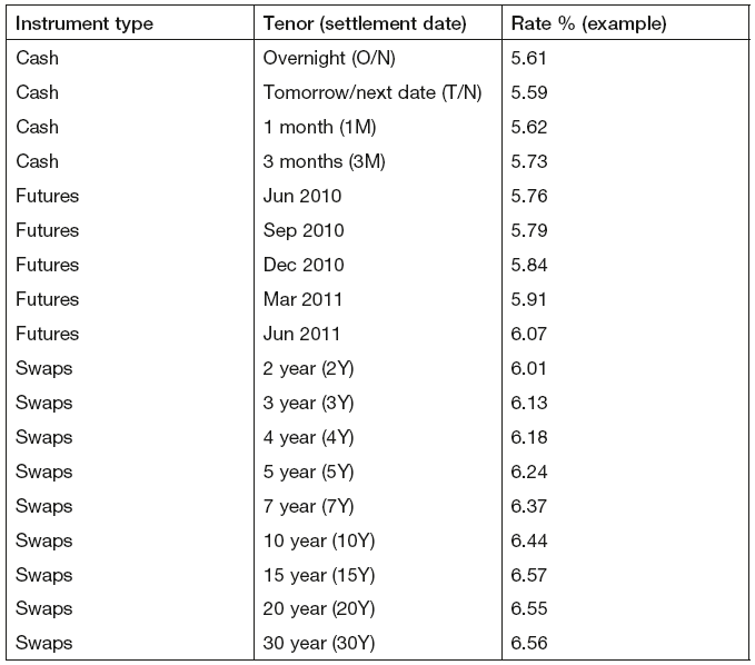
Futures take precedence over all other instruments. The point at which futures take over from deposits and the number of futures used in each curve depends on the currency and instruments being priced. A typical yield curve would consist of the grid points shown in Table 14.1.
Table 14.1 Standard yield curve grid points
Standard curves typically model three-month borrowing rates (three-month Libor in the UK), to be used for pricing instruments of all maturities. This choice is based on the fact that should the bank require funding to cover its position it would borrow at those rates. However, some market practitioners prefer pricing short-tenor instruments off a curve that models one-month interest rates (as they would typically only borrow funds in the market for a short period of time). To meet these requirements two curves are typically constructed for each currency:
- Three-month curve
- One-month curve.
The three-month curve construction methodology tends to use deposits, futures and swaps.
The one-month curve typically uses deposits and futures, as there is no need to include points at longer tenors, thus omitting swaps.
In addition to the above curves, a basis curve is often constructed and used to price cross-currency instruments. This curve models the market prices of such instruments more closely than the Libor curve as it captures the true cost of funding.
The methodology for all the above curves is described in subsequent paragraphs.
YIELD CURVE CONSTRUCTION METHODOLOGY
The three-month yield curve construction
As was stated earlier, the three-month curve is built using:
- Deposits
- Futures
- Swaps.
Deposits
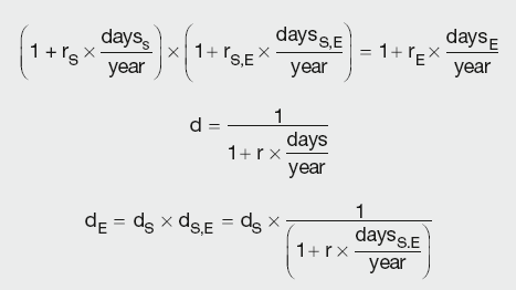
Deposit (cash) rates are used until the first future or FRA contract becomes available. Discount factors are generated for the maturity date of each point in the curve using the equation for forward-forward rate and the relationship between the rate and the DF:
Calculation Summary: Yield curve discount factors derived from deposit rates
where:
year is the number of days in the year
daysS, daysE and daysS,E are the relevant time periods
dS and dE are the discount factors for the period start and end date
dS,E is the discount factor for the period daysS,E
rS and rE are the spot rates for the period start and end dates
rS,E is the interest rate for the period daysS,E.
Futures
The relationship between the futures implied rate and the quoted price is f = (100 – p)/100 + adj, where f is the forward rate for the period starting at futures expiry date (expressed as a percentage) and adj is convexity adjustment (described below). As futures rate is given by:
Calculation Summary: Futures rate as a function of start and end period discount factors
where:
daysS,E is the time period covered
dS and dE are the discount factors for period start and end dates.
The DF for the end of the forward period can be calculated by rearranging the above equation:
Calculation Summary: Yield curve discount factors derived from futures prices

Thus, the DFs at the end of each forward period can be calculated from the relevant futures price and the DF at the beginning of that period. Hence, the discount factor at the start date of the first future has to be known, i.e. the settlement date of the first futures contract should lie before the maturity date of the last deposit rate (thus it is necessary to include at least two cash rates into the curve).
A futures contract that settles at time t1 (spanning the period from t1 to t2) that lies between two cash rates (e.g. 1M and 3M) gives two options for DF interpolation:
- Interpolating DF1 for t1 directly from DFs for 1M and 3M
- Interpolating rate at t1 from 1M and 3M cash rates, and then deriving DF1.
The decision on which method to use is simply a matter of choice.
Futures convexity adjustment
As discussed in Chapter 6, a FRA is sensitive to two rates:
- The forward rate that determines the payment.
- The spot rate that determines the DF used to calculate the present value of the cash flow.
In contrast, a future price is only sensitive to the forward rate as the variation margins are paid daily. Thus, the relationship between the future payoff and forward rate is linear, whereas it is convex for FRAs. Although this convexity effect is small at the short end of the yield curve, it becomes more significant as the maturity increases. As this is recognised by market practitioners, the implied futures rate is higher than the equivalent IMM FRA. This difference is often called convexity. As a market convention, convexity adjustment is defined as the difference between the futures rate and the FRA rate. Consequently, the curves using futures prices for construction incorporate this adjustment.
Swaps
As futures contract for longer tenors become less liquid they are substituted by swaps. The general equation for the DF of the last swap coupon payment will be deduced from an example of a two-year annual swap, where the present value (PV) of the future cashflows is calculated as the difference between the fixed and the floating legs:
where:
P is the notional principal
dk is the discount factor for the end of period k, implying d0 = 1
daysk is the number of days in the coupon period k
Lk–1,k is Libor for that period
C is the fixed coupon rate for the duration of the swap.
As the interest rate r implied by the DFs for adjacent periods, calculated as:

is equivalent to the Libor rate for that period; substituting Lk–1,k for rk–1,k and d0 with 1 reduces PV(floating) to:
PV(floating) = P × (1 − d2)
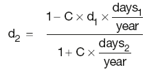
Thus d2 can be calculated by rearranging the above equation:
Hence, calculation of d2 requires knowledge of d1.
The above equation can be generalised to give the discount factors for all subsequent points:
Calculation Summary: Yield curve discount factors derived from swap rates
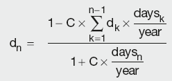
It is clear that in order to apply the above expression, all the swap rates and the DFs associated with all but the last payment date have to be known or otherwise interpolated. This process (known as ‘bootstrapping’) is performed in ascending order of maturity, commencing with the first point in the swap strip.
Bootstrapping the swap strip
If only the last discount factor (dn) in the swap strip is unknown, it can be calculated directly from the last equation. However, if there are two or more DFs then all unknowns must be solved for simultaneously using iterative approximation.
The method of calculation of DFs for new swaps in the curve depends on the frequency of the two swap legs as well as the presence of the synthetic swap DFs (linearly interpolated from the market values). Synthetic DFs are typically introduced when the fixed leg has a higher frequency than the floating leg, so that the values at those intermediate points are readily available.
The following summarises all possible cases:
Fixed and floating leg frequency is the same: Each new swap introduces only one unknown (dn) which is calculated directly from the last equation.
Different frequency, synthetic DFs available: The fixed leg payment rates can be derived from market data (used to calculate intermediate DFs, as described above), hence the case is directly solvable as above.
Different frequency, no synthetic DFs: The first market-quoted swap maturity is too far away from the last future contract and intermediate DFs are needed. This generates several unknown DFs that must be solved for simultaneously using iterative approximation. In this case, the first DF in the swap strip (beyond the futures strip) can be calculated by interpolating between the last future and the first market-quoted swap, repeating the process for all required points.
Two alternative interpolation methods that can be used for bootstrapping are described below.
Interpolation methods
Zero-rate linear interpolation
Zero-rate is the interest rate prevailing between two dates assuming that all the interest is paid at maturity. As zero-rate is a continuously compounded rate, it relates to DF and the spot rate as:

which, when rearranged, gives:

The unknown zero-rate zx is interpolated by fitting a straight line between the two adjacent points z1 and z2:
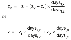
By substituting into the above equation, the DF for the unknown point can be calculated as:
Calculation Summary: Linear interpolation of yield curve discount factors
where the symbol ^ denotes ‘power of ’.
Log-linear interpolation
Log-linear (geometric) interpolation assumes that the continuously compounded interest rate over any period within the given time interval t1 to t2 is the same as the continuously compounded rate over the entire period. Hence, using the same notation as above, the unknown DF can be calculated as:
Calculation Summary: Log-linear interpolation of yield curve discount factors
which can be rearranged into:
THE ONE-MONTH YIELD CURVE CONSTRUCTION
Curve instruments
One-month curves are used by market practitioners to price short-term instruments (particularly those with one-month tenors). Since these instruments do not require long-term rates, the curve construction typically omits swaps and is based on:
- Deposits
- Futures/IMM FRAs
Curve construction
Constructing the one-month curve is much simpler than the process required by the three-month curve. As the curve only covers the short period, there is always sufficient market data for the calculation of DFs. Given that the periods covered by the interest rates are short, all the market rates rk can be converted into continuously compounded rates zk using:

Regardless of whether the deposit or future/FRA rate is used, the one-month rates can be calculated from the available market data using an expression akin to the futures or FRAs strip rate:
Calculation Summary: Derivation of one-month rates from available market rates

In other words, the effect of compounding the one-month rates has to be the same as the original continuously compounded rate. This is typically achieved by iteratively adjusting the rates until conversion criteria are reached.
The above procedure is repeated for all market rates used in the curve, thus obtaining a series of one-month rates for different tenors. They are used to calculate DFs as follows:
Calculation Summary: One-month curve discount factors derived from one-month rates
where:
year is the number of days in the year
daysS,E is the time period covered by one-month rates
zS,E is the continuously compounded one-month rates for that period.
THE BASIS CURVE CONSTRUCTION
Introduction
The underlying assumption behind the three-month and the one-month curves described in the previous sections is that the funding rate prevailing in the market is Libor (or equivalent for a given currency). This is the rate used to represent floating rate funding as well as calculating DFs. However, not all market practitioners have access to Libor funding, particularly in cross-currency transactions.
Hence a curve – called a basis curve – that represents a true cost of funding is needed.
Basis curve methodology
The basis curve is typically constructed using deposits and swaps. The futures, as exchange-traded instruments, do not incur additional financing costs; hence they are replaced by swaps of shorter maturities in order to close the gap after the last deposit contract.
Thus the basis curve DFs are calculated as follows:
- Short-end DFs are calculated from the Libor rates increased by market-implied spread, to reflect the true cost of funding (basis).
- Medium-term DFs are calculated from swaps, by adding the predetermined spread to the Libor rates implied by futures.
- For long-term DFs, two unknown quantities (dn and Ln) are introduced for every new point and are calculated by simultaneously solving the basis and Libor curves.
The sections below describe this process in more detail.
Short-term rates (deposits)
The basis curve deposit discount factors are calculated using the following expression (slight modification of the Libor curve approach):
Calculation Summary: Basis curve discount factors derived from deposit rates

where:
r is the prevailing Libor rate
b is the estimated basis
daysS,E is the time perio S,E d covered
dS and dE are the discount factor S E s for the period start and end dates
dS,E is the discount factor for the period daysS,E
rS and rE are the spot rates for the period start and end dates
rS,E is the interes rate the period daysS,E.
Medium-term rates (swaps)
To compensate for the lack of futures in the medium-term part of the curve, swaps of shorter maturities are used. However, they are not incorporated in the same way as for three-month Libor curve. As Libor rates are known at these maturities (as implied by the futures used in the Libor curve), dn for every new swap point can simply be calculated from:
Calculation Summary: Basis curve discount factors derived from medium-term swap rates
using know Libor rates Lk and predetermined basis bn.
Each basis curve can have one or more Libor curves, used for calculating floating swap legs, associated with it.
Long-term rates (swaps)
As the Libor curve is used for calculating floating leg cashflows, and the basis curve is used for discounting, each new swap point needs to satisfy both curves, i.e. the vanilla swap equation:
and the basis swap equation:
where:
daysk is the number of days in the coupon period k
C is the fixed coupon rate for the vanilla swap
Lk–1,k is the Libor for the period k
bn is the basis over Libor for the particular swap.
The summation factors i, j and k are deliberately different to account for different leg frequencies of different swaps and their individual legs.
Rearranging the second equation and substituting the first into it, gives:
Calculation Summary: Basis curve discount factors derived from long-term swap rates
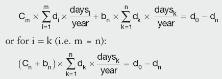
The bootstrapping procedure is exactly the same as for the three-month curve, solving directly if only one dn is unknown, or simultaneously for more than one DF.
SHAPE OF THE YIELD CURVE
There are several theories behind the yield curve shape:
- The pure expectations theory states that the only determinant of the yield curve shape is investors’ expectations of future short-term interest rates.
- The liquidity preference theory is based on the assumption that the investors expect to be compensated for having their funds tied up for long periods, requiring ever increasing yields for longer maturities
- The preferred habitat theory is similar to the above, implying that investors expect higher returns for longer maturities, as they are associated with more risk. However, the risk arises from liquidity of the longer-term securities (as most investors plan short and medium term), rather than purely from maturity.
Because the yield curve can reflect investors’ expectations of interest rates, inflation, political and economic events as well as the impact of risk premiums for longer-term investments, interpreting the yield curve is complicated. Market practitioners put great effort into trying to understand exactly what factors are driving the yields.
Normal yield curve
A normal yield curve implies that yields rise with maturity (i.e., the slope of the yield curve is positive). This reflects market expectations of economic growth and increased inflation in the future. The typical response of central banks in such a scenario is raising short-term interest rates to encourage saving, rather than spending. There is also uncertainty associated with estimates of future interest rates and the funds put on long-term deposit. Investors price these risks by demanding higher yields for maturities further into the future.
Steep yield curve
Extending the logic from the above, the steep yield curve implies market expectations that the economy will grow at faster rate in the future than in the current period, such as at times of expansion.
Flat or humped yield curve
When all maturities have similar yields, a flat yield curve is observed. This implies uncertainty in the economy, whereby the market participants are holding off their investment decisions until the situation clarifies. Another possibility is a humped curve, created when medium-term yields are higher than those of the short term and long term. This typically implies market expectation of rapid economic growth in the short term with more uncertainty in the future.
Inverted yield curve
The inverted yield curve represents market expectation of worsening economy. In addition to economic decline, inverted yield curves also imply that the inflation is likely to remain low.
GRAPHICAL YIELD CURVE REPRESENTATION
The above curve construction methodologies are implemented as computer software which generates curves for each currency. Their output is typically a range of discount factors (DFs) for selected dates. If a DF is required for a non-grid point, interpolation is used to provide the rate or DF for that date. But the curves are often represented graphically to give some idea of market expectations, with the tenors on the x-axes and yields on the y-axes.

