Notation

Time value of money

Money markets calculations

Capital markets instruments

Financial futures

Forward rate agreements (FRAs)

Interest rate swaps

Foreign exchange

Option characteristics

Option pricing

Bond derivatives

Equity derivatives

Probability and statistics

Yield curves

NOTATION

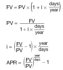
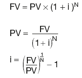
i	annual interest rate
n	number of payments per year
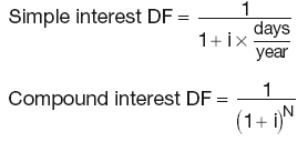
days	number of days in the investment/coupon period
year	number of days in a year
N	number of years or coupon periods
P	price
APR	annual percentage rate, effective rate or equivalent annual rate
PV	present value
FV	future value
DF	discount factor

TIME VALUE OF MONEY

Effective and nominal rates

Relationship between the interest rate i with n payments per year and the APR:

Continuously compounded rate

where i is the nominal interest rate.

For annual effective rate APR:

r = ln(1 + APR)

Reinvestment rates

For unequal rates applying to different investment periods:

Short-term investments

Long-term investments

Discount factors

NPV and IRR

Internal rate of return (IRR) is the rate that discounts all the cashflows, including any cashflow now, to zero.

IRR discounts all the future cashflows to a given NPV.

MONEY MARKETS CALCULATIONS

Certificate of deposit (CD)

Proceeds at maturity:

Secondary market yield:

Discount instruments

Proceeds at maturity:

Maturity proceeds P = F(face value)

Secondary market price:

CAPITAL MARKETS INSTRUMENTS

Simple bond dirty price formula

where:

C_k is the k^th cashflow (including the final redemption amount)

i is the bond yield, based on the payment frequency

n is the number of coupons per year

d_k is the number of days until the k^th cashflow.

Accrued coupon

where d_cs is the time period between the last coupon date and the sale of the bond.

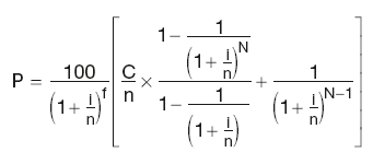
Clean bond price

where:

C is the annual coupon rate

N is the number of outstanding coupons

i is the annual bond yield, based on the payment frequency

n is the number of coupons per year

f is the ratio between the number of days until the next coupon and the full coupon period.

Ex-dividend

where:

d_pc is the time period between the bond purchase and the next coupon.

Bond yield

Flat yield:

Flat yield = (Coupon rate/Clean price) × 100

Simple yield to maturity:

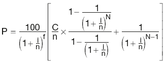
Yield accounting for coupon payments and irregular first coupon period (derived from the pricing formula):

where:

C is the annual coupon rate

N is the number of outstanding coupons

i is the annual bond yield, based on the payment frequency

n is the number of coupons per year

f is the ratio between the number of days until the next coupon and the full coupon period.

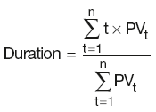
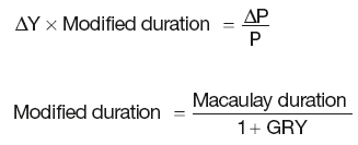
Portfolio duration

Macaulay duration:

Modified duration:

FINANCIAL FUTURES

Futures price

Price = 100 – Implied forward interest rate × 100

Futures settlement price

Expressed in terms of ‘ticks’:

Profit/Loss = Tick movement × Tick size × Number of contracts

Futures strip rate

FORWARD RATE AGREEMENTS (FRAs)

FRA rate

where:

i_L is the interest rate for the longer period

i_S is the interest rate for the shorter period

d_L is the number of days in the longer period

d_S is the number of days in the shorter period

year is the number of days in the year.

FRA settlement price

where:

f is the FRA interest rate

d_f is the number of days in the FRA period

year is the number of days in the year.

INTEREST RATE SWAPS

Short-term swap valuation at inception

where:

r_S is the swap rate

days_k is the number of days covered by the k^th FRA contract

DF_k is the discount factor derived from the k^th FRA rate f using:

Later valuation of short-term swap fixed leg

where:

P is the value of the fixed leg at a later date

r_S is the swap rate, fixed at inception

days_k is the number of days covered by the k^th FRA contract

DF_k is the discount factor derived from the k^th FRA rate f_k using:

FOREIGN EXCHANGE

Spot rates

Given exchange rates X/Y and X/Z, the cross-rates are:

and

Given exchange rates Y/X and Z/X, the cross-rates are:

and

Given exchange rates Y/X and X/Z, the cross-rates are:

and

Forward outrights

where:

FX_f is the forward exchange rate

FX_s is the spot exchange rate

r_v is the interest rate applicable to variable currency

r_b is the interest rate applicable to base currency.

Forward swaps

Forward swap = Forward outright – Spot

where:

FS is the forward swap price

FX_f is the forward exchange rate

FX_s is the spot exchange rate

r_v is the interest rate applicable to variable currency

r_b is the interest rate applicable to base currency.

Cross-rate forwards

Given forward exchange rates X/Y and X/Z, the forward cross-rates are:

and

Given forward exchange rates Y/X and Z/X, the forward cross-rates are:

and

Given forward exchange rates Y/X and X/Z, the forward cross-rates are:

and

Cross-rate forward swaps

Given spot exchange rates X_s/Y_s and X_s/Z_s and forward exchange rates X_f/Y_f and X_f/Z_f, the forward cross-rate swap prices are:

Given exchange rates Y/X and Z/X, the forward cross-rates are:

Given exchange rates Y/X and X/Z, the forward cross-rates are:

OPTION CHARACTERISTICS

Put-call parity

C − P = S − K

where:

C is the call premium, P is the put premium

S is the futures price, K is the exercise price/option strike.

Physically settled options

C − P = S − Ke^–rt

where:

r is the continuously compounded interest rate

t is time to expiry expressed as .

Options on dividend-paying stocks

C − P = S − Ke^–rt − D

where:

D is the present value of the expected dividend.

Options on stock index (dividend yield continuous)

C − P = Se^–dt − Ke^–rt

where:

d is the continuously compounded dividend yield.

Cross-currency options

C − P = Se^–ft − Ke^–rt

where:

f is the continuously compounded foreign currency interest rate

S is the spot exchange rate.

Options on futures with up-front premiums

C − P = S − K

Options on futures with margined premiums

C − P = Se^–rt − Ke^–rt

Option value sensitivities – ‘option Greeks’

Options sensitivity to	Named as
Underlying	Delta
Changes in delta	Gamma
Volatility	Vega or kappa
Time decay	Theta
Interest rates	Rho

OPTION PRICING

Risk-neutral pricing using binomial trees

Call option premium boundaries:

Probability-weighted stock price

Pricing options using hedge ratio

where:

Dividend paying stock options

Cross-currency options

Option pricing using Black–Scholes

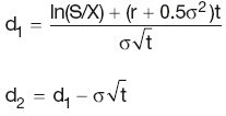
Black–Scholes model:

where:

and

S is the underlying stock/share price

X is the exercise price

r is the annual continuously compounded risk-free rate

t is the time (in years)

σ is the annual stock price volatility

N(d) is the cumulative probability that deviations less than d will occur in a normal distribution with a mean of 0 and a standard deviation of 1

N(d₁) is the probability of the stock price rising to a certain level

N(d₂) is the probability of the stock price rising above the strike (but it is irrelevant by how much).

Options on futures (premiums paid up front)

Options on futures (premiums margined)

Currency options

Black model

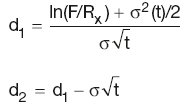
Black model for interest rate derivatives:

where:

where F is the current market forward swap rate, and R_x is the underlying swap rate (option strike). All other variables have the same meaning as before.

BOND DERIVATIVES

Bond futures

Deliverable bond valuation:

Bond futures price:

Forward bond price:

Bond repos

where r is the repo rate and days refers to number of days until maturity.

Bond options

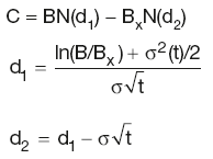
Black model for bond options:

Put–call parity for bond options:

F is the futures price

K is the exercise price/option strike

r is the continuously compounded interest rate.

EQUITY DERIVATIVES

Equity index futures

The futures settlement price:

Equity index futures price:

where:

i is the annual funding rate

d is the dividend yield on underlying equity.

Stock beta

Portfolio beta:

where:

β_i is the individual equity beta

V_i is the individual equity share value

V_P is the total value of the portfolio.

Equity index options

Black–Scholes for equity index options:

where dividend yield d is assumed to be paid continuously.

Put-call parity for equity index options:

Single stock options

Black–Scholes for single stock options:

where dividend payments until expiry are captured by reducing the stock price by the present value of dividends.

Put–call parity for dividend-paying single stocks:

C − P = S − D − Ke^−rt

where D is the present value of expected dividend.

Equity index swap valuation

PV(swap) = PV(equity index leg) − PV(floating leg) = 0

PROBABILITY AND STATISTICS

Main concepts of probability

Probability of an event E when there are several equally likely outcomes:

P(E) = Number of ways E can occur/Total number of possible outcomes

Sample-based probability:

P(E) = Number of observed occurrences of E/Total number of observed occurrences

Joint probability

Independent events:

Dependent events:

Probability distribution

Probability that the continuous variable x has a value between a and b inclusive:

Probability that the discrete variable x has a value X or lies between a and b inclusive:

Probability that the continuous variable x has a value less than or equal to X:

Probability that the discrete variable x has a value less than or equal to X:

Binomial distribution

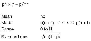
Binomial probability function:

where the number of possible combinations of x successes in n trials is given by:

and the probability of x successes and n – x failures in a trial is given by:

Normal distribution

Normal distribution function:

Standard normal distribution function:

Mean	location parameter μ
Median	location parameter μ
Mode	location parameter μ
Standard dev.	scale parameter σ

Log-normal distribution

Log-normal distribution function:

Standard log-normal distribution function:

YIELD CURVES

Choice of instruments

1. Cash deposits.
2. Interest rate futures.
3. Interest rate swaps.

Deposit discount factors

The forward–forward rate is given by:

and the relationship between the rate and the DF is:

Hence it follows:

where:

year is the number of days in the year

days_S, days_E and days_S,E are the relevant time periods

d_S and d_E are the discount factors for the period start and end date

d_S,E is the discount factor for the period days_S,E

r_S and r_E are the spot rates for the period start and end dates

r_S,E is the interest rate for the period days_S,E.

Futures discount factors

Given the futures rate:

the DF for the end of the forward period is given by:

Swap discount factors

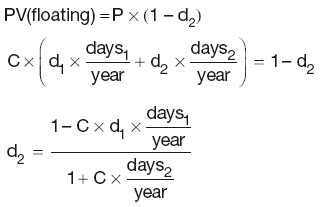
where:

P is the notional principal

d_k is the discount factor for the end of period k, implying d₀ = 1

days_k is the number of days in the coupon period k

L_k-1,k is the Libor for that period

C is the fixed coupon rate for the duration of the swap.

As the interest rate r implied by the DFs for adjacent periods can be calculated as:

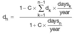
It follows:

In general:

Interpolation methods

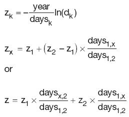
Zero rate linear interpolation:

which, when rearranged, gives:

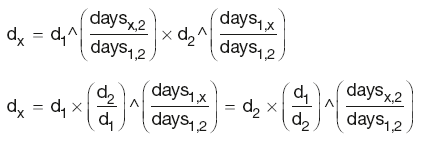
DF for the unknown point can be calculated as:

where the symbol ^ denotes ‘power of ’.

Log-linear interpolation