
Chapter 8
Radio Mobile Measurement Techniques1
8.1. Introduction
Propagation measurements allow us to better understand the different propagation mechanisms (reflection, transmission, diffraction, scattering, guiding) and to characterize the propagation channel in the considered environments (urban, suburban, rural, mountainous, inside buildings, etc.) for better models and predictions. This modeling is necessary for the conception of telecommunication systems and, once they have been designed, for their actual field deployment.
In the first case propagation models are implemented in software in order to simulate the transmission chain. These models are based on the consideration of the impulse response and its evolution in space and time and rely on generic or typical environments rather than on geographical databases.
In the second case propagation models are implemented in engineering tools for the prediction of different parameters useful for the field deployment of systems, for the study of radio coverage (selection of emission sites, frequency allocation, powers evaluation, antenna gains, polarization, etc.) and for the definition of the interference occurring between distant transmitters.
So, different measurements methods are managed as a function of analysis and model requirements: narrowband measurements (field strength measurements), broadband even ultra wide band measurements (impulse response measurements), direction of arrival measurements and transmission rates.
For each of these different measurements techniques, the associated treatments are detailed by putting more emphasis on mobile radio communications.
The different sections hereafter are the result of work completed by France Telecom R&D on the one hand, and a compilation of a bibliographic work on the other hand.
8.2. Field strength measurements
In narrow band, the frequency band used is lower than the coherence band (CB). A narrow band signal is therefore characterized by quasi-constant amplitude inside this band of frequency. So, only attenuation and its variations are sufficient to study the propagation channel. In order to compensate for the possible increase of attenuation, we generally resort in analog to the use of a power margin, and in digital to frequency hopping.
Narrow band measurements allow the study of attenuation by the elaboration of field strength models and the study of the statistics of the instantaneous field (Rayleigh law, Rice law, etc.). Models are of different types. We distinguish theoretical or deterministic, empirical and semi-empirical models.
Theoretical models are based on the fundamental laws of physics combined with adequate approximations and with atmosphere, land or building data bases (ray tracing, ray launching model).
Empirical models are based on the statistical analysis of a large number of experimental measurements conducted with respect of several different parameters like the frequency, the distance, the effective heights of the base station antenna and of the mobile, etc. The best known model is the Okumura-Hata model, which is based on the statistical analysis of a large number of experimental measurements conducted inside and near Tokyo, with respect to different parameters like the frequency or the distance.
Semi-empirical models combine the analytical formulation of physical phenomena like reflection, transmission, diffraction or scattering with a statistical fitting by variable adjustment using experimental measurements.
Prediction models of the field strength are used for determining the radio coverage of the emitters, i.e. to predict the local average value of the envelope of the electric field at a given point. Measurements conducted in different environments allow the development as well as the statistical optimization and the validation of these models. These measurements allow us to record both the instantaneous and the average value over a short time interval of the radio field strength along a path travelled by a mobile , or in this case by a vehicle.
Figure 8.1. Measurement principle of the mobile radio field strength
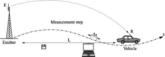
The measurement principle (Figure 8.1) is summarized as an emitting station implementing, at a given site, beams in the space electromagnetic wave amplitude and frequency which are constant in time (carrier). A vehicle (or a wagon in the case of measurements carried out indoors) equipped with a field intensity measuring device and a data acquisition receiver moves along a definite set of paths. An impulse generator bound to one of the wheels of the vehicle engages measurements of the instantaneous field. The measurements are taken at fixed distance intervals rather than at fixed time intervals, since this would force the vehicle to move at a constant speed and cannot be easily be achieved in practice in urban environments. This distance interval (Δx) is called the spatial sampling step or the measurement step. The computer controlled receiver is coupled to a data acquisition system and magnetic storage system of the field strength measured in dBμV/m
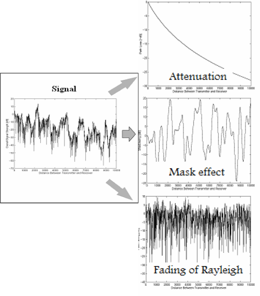
A numerical analysis is then performed in order to associate geographical coordinates with each measurement point. This operation is achieved using either a chart with a digitizer, or a geographical database with digitization software. In general, real-time localization systems such as the GPS system do not authorize the capture of the geographical coordinates with a sufficient degree of precision, more particularly in urban environments where it should be lower than 1 m. The measurements thus performed are said to be raw: they reproduce all the variations affecting the amplitude of the signal, in proportion to the envelope of the electric field. A data analysis associated with a numerical filtering is then performed in order to eliminate the fast variations due to Rayleigh fading from the slow medium-scale variations which can be modeled and predicted.
Figure 8.2. Example of the variation of radio electrical signal according to the distance performed by the mobile, superimposing of slow variations of great (due to distance), medium scale (due to mask effects) and quick variations (Rayleigh fading)
The spatial sampling step (Δx) of the data acquisition system is selected so as to allow the reconstitution of the signal. The Nyquist theorem imposes a sampling no higher than λ/2, where λ is the wave length of the wave beamed by the emitter station. The average length L of the interval must be selected such a way as to minimize the local average error of the envelope of the radio field. The mobile radio signal being assumed to be, in wide sense, stationary over the average interval length, the latter must be higher than the maximum distance at which the local average can be regarded as constant. This maximum distance is a function of the local average distribution depending on the environment, which itself depends on the frequency. As an example, the effects induced by diffraction are more pronounced when the frequency increases. The sampling step is therefore empirically determined with respect to the environment (rural, mountainous, suburban, inside of buildings, etc.) and to the frequency. In general an average length L equal to 40 λ is used. The local average value of the mobile radio signal is then estimated to more or less 1 dB in 90% of cases (Lee, 1986).
Figure 8.2 gives an example of the variation of a radio electrical signal according to the distance performed by the mobile, superimposing of slow variations of great (due to the distance), medium scale (due to mask effects) and quick variations (Rayleigh fading).
8.3. Measurement of the impulse response
In broadband, the frequency band used is greater than the CB. The presence of multiple paths leads to the temporal spreading of the received signals, revealed by the presence of power peaks in the impulse response, and to a major fading in the frequency domain. The different spectral components of the emitted signal are not affected in the same way over the used frequency band. This phenomenon, associated with the temporal spreading of the signal, results in the appearance of inter-symbol interferences due to the superposition of the delayed preceding symbols on the last emitted symbol. The possibility that such inter-symbol interference may occur imposes a higher limit to the bit data rate. This limit can be improved if an equalizer is used.
The methods used for measuring the impulse response of a system can be classified into two families: frequency methods and temporal methods.
Frequency methods measure the path loss in a given frequency band by performing a frequency scan. The intrinsic difficulty of these methods lies in obtaining the phase of the impulse response. The most commonly adopted methods, used for instance in networks analyzers, consists of synchronizing with a cable the transmitter and the receiver. The impulse response is obtained by the Fourier transform. Frequential methods are more specifically adapted to the characterization in broad frequency range of the propagation of millimeter waves inside buildings (Jimenez, 1994).
Two different types of temporal methods exist:
– The simplest method is based on the transmission of a very short impulse as close as possible to a Dirac function. The instantaneous field measured at the reception point directly corresponds to the impulse response of the radio channel. Although this method is simple in theory, in practice its implementation turns out to be complicated: not only is it difficult to emit high power impulses in a very short time, but the reception of such impulse is delicate (Kauschke, 1994).
– A second method consists of using a sounding signal in the form of a pseudorandom binary sequence with good autocorrelation properties and with a maximum length. This sequence modulates a carrier signal, which generally has a BPSK modulation type. The correlation of the received sequence with an image of the emitted sequence is then performed by the receiver: due to the autocorrelation property of sequences with maximum length sequences, a correlation peak can thus be obtained. Channel sounders with analog sliding correlators have also been used: however, these sounders were limited, most of all because they did not provide the phase information (Parsons, 1992). It is indeed essential, especially in the case of hardware and software simulations, to determine the amplitude and phase of the impulse response. With the advances in numerical analysis methods, recent sounders use, in the presence of noise, digital processing related to inversion methods like the Wiener inversion. The use of such digital processing also allows us to achieve both a higher resolution and a lower sensitivity to the non-linearities in the transmission chain. Several different systems have been developed according to this method (Kauschke, 1994), (Levy, 1990), (Zollinger, 1988), etc. The reader will find a more extensive bibliography in Vu (2005), Pagani et al. (2009) and in the COST 231 final report (COST231, 1999).
The main characteristics of a propagation channel sounder are as follows:
– The analysis band is defined as the frequency band around the central frequency at which the measurement is performed. The analysis band must be higher than the frequency band planned for the useful signal. The wider the frequency band is, the better the temporal resolution of the sounder is, i.e. the possibility of separating close delays. Analysis bands typically range from approximately a few megahertz to several tens of megahertz.
– The maximum length of the impulse response in mountainous environments is the maximum delay due to remote echoes, which may reach an order of a few tens of microseconds (1 μs corresponds roughly to a 300 meter path).
– The spatial or temporal sampling step which corresponds to the width of the analyzable Doppler spectrum. This width is inversely proportional to the time interval separating two successive impulse responses.
– The measurement dynamics, which can be expressed through the relation between the power of the strongest path and the noise threshold. The dynamics generally obtained with present day propagation channel sounders are of the order of 30 dB.
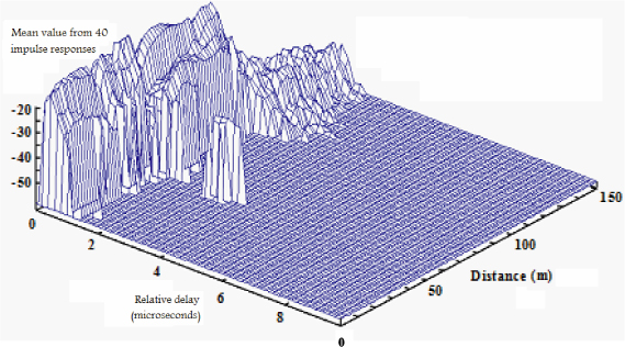
Figure 8.3 presents an example of the variation of the impulse response in a microcell context of a mobile turning at a street corner. The received power is reduced from 30 dB and the form of the response is significantly changed.
Figure 8.3. Evolution of the impulse response at a street corner in a microcell environment (Paris, 900 MHz, France Telecom R&D sounder)
In order to conduct studies on propagation as well as set up the models integrated to the radio engineering devices, France Telecom R&D defined and developed, in its laboratories in Belfort, a propagation channel sounder called AMERICC (Appareil de mesure de réponse impulsionnelle pour la caractérisation du canal radio – impulse response measurement system for characterization of radio channels). This device allows a more accurate characterization of the radio propagation channel over a bandwidth ranging from 0 to 250 MHz around a carrier frequency ranging from 1.9 to 60 GHz (Conrat, 2002).
This sounder can be used for the characterization of the different multiple paths with regard to their lengths, directions of arrival (DOA), amplitudes and phase terms. This very complete characterization of the propagation channel allows us to define with great precision, the quality of future communication systems (UMTS, LMDS, WiFi, WIMAX, MIMO, etc.) and is absolutely essential for the development of realistic propagation models for the study of multiple-input multiple-output (MIMO) radio communication systems.
The technical features of this sounder include:
– a sensibility of the order of -85 dBm;
– a dynamic greater than 40 dB;
– a space resolution of the order of 1 m owing to its data acquisition system at the 1 GHz frequency;
– a multi-sensor array system with ten antennas at the reception point;
– a carrier frequency adjustable from 1.9 GHz to 60 GHz;
– GPS positioning and remote piloting.
There are numerous different channel sounder types (SISO, SIMO, MIMO, PRS, etc.), in different frequency bands and using different processing techniques (Fast Fourier Transform, ESPRIT, SAGE, MUSIC, etc.) in the literature: Scipio (high frequency), (Vu, 2005), Pastel, LST, (Zayana, 2003), Medav, Electrobit, etc.
The conversion of a SIMO sounder in a UWB sounder uses the duality between multi-sensors measurement and multi-frequency band measurement. The multisensor fast communication system is used for the synchronous switching of the carrier frequencies of each partial band to be measured (Pagani, 2008). The reader will also find a list of UWB radio channel measurement campaigns created using different sounder techniques.
8.4. Measurement of directions of arrival
The use of multi-sensors antennas and MIMO (multiple input/multiple output) techniques improve radio mobile networks:
– reducing the number of base stations necessary to the coverage of weak traffic areas;
– improving the radio coverage that can allow better buildings penetration;
– power distribution;
– radiation patterns orientation in direction of specific users;
– orientation of zero radiation patterns in the direction of interfering emitters;
– increase capacity in fixed base stations number, in a great traffic microcell environment.
These different techniques exploit the possibilities of using the different electromagnetic wave propagation paths existing between the transmitter and the receiver. So DOA of such waves are necessary. The knowledge of DOA allows us to better comprehend the propagation environment and model the propagation channel. It registers in the programs of propagation modeling by ray tracing or ray launching techniques
These measurements are intended to evaluate the angular distribution of the received energy, i.e. determining the arrival direction of the waves. The simplest idea consists of using a very directive rotating antenna. This however cannot be achieved at these frequencies (1–5 GHz). Although the use of a multi-sensor array antenna would be an ideal solution, its implementation would require N parallel measurement chains. Therefore, a simulated antenna array consisting of a rotating arm device coupled to a reference antenna is used in practice for the measurement of DOA. The environment is assumed to be stationary during the rotation time of the arm. This measurement can be demonstrated to be equivalent to a multi-sensor measurement along a circular antenna array.
In a narrow frequency range, the signal is subject to Rayleigh fading: therefore, no privileged direction of arrival of the signal can be identified at these frequencies, whereas in a broad frequency range, the instantaneous power is subject to greatly attenuated fast variations resulting from the frequency selectivity of the channel. This method is therefore generally adopted (Rossi, 1997).
The results, presented in the form of polar diagrams with an amplitude scale expressed in dB, allow us to validate prediction models of the field strength, using for instance the profile method or the ray launching method. A better understanding of the angular distribution of energy at the level of the base station enables the development of new spatial techniques based on the use of adaptive antennas: like the beam-forming method or the spatial division multiple access (SDMA) method (Guisnet 1996; Klein 1996; Thomson 1996; Ertel 1998; Guisnet 1999; Pajusco 1998).
More details on the subject of DOA – their experimental determination, their mathematical modeling as well as their different linear and high-resolution determination methods of the DOA – will be provided in the following sections.
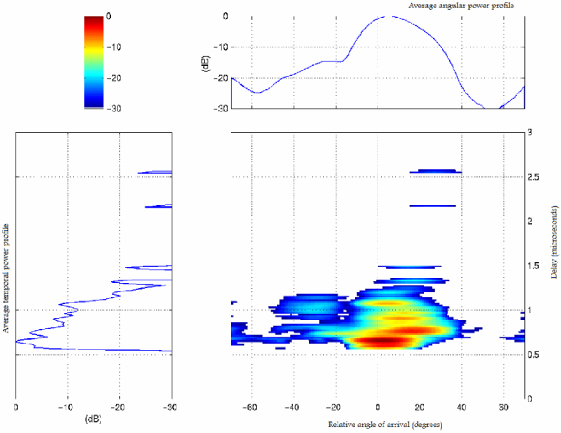
Figure 8.4 presents an example of the spatial-temporal representation of the complex impulse response measured during a broadband multisensor experiment undertaken in a dense environment at 2 GHz frequency and in small cell environment (antenna located above the roof level) (Laspougeas, 2000).
Figure 8.4. Spatial-temporal representation of the impulse response in a configuration with average temporal and spatial selectivity: Angular power profile, temporal power profile, average spatial-temporal power distribution. The origin of the angles corresponds to the pointing axis of the base station antenna
8.4.1. Mathematical modeling of the signal
In broad frequency range, the received signals arrive at the antenna array with a delay τ. If Δτ is the time resolution of the impulse response, then the matrix containing the direction of arrival information is only weakly time-dependent, provided however that Δτ satisfies the following condition: r0/c which is very small comparing to Δτ.
The time resolution Δτ of the impulse response is directly dependent on the frequency band B for which the impulse response was evaluated, as shown by the following equation:
![]()
Let us here consider an array of M antennas distributed regularly along the circumference of a circle with radius r0. Let us then assume that a given emission source has been chosen and that N multiple paths arrive at the antenna array. It shall be further assumed that the multiple paths correspond to vertically polarized plane waves arriving at the antenna array with an elevation φn and an azimuth θn. The channel sounder performs measurements at a constant angular step along the circle described by the omnidirectional antenna at the angles 2π m / M, where m ∈ {0, 1, …, M − 1}.
Figure 8.5. Circular antenna array
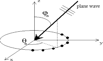
In far field assumption, the field received by the mth antenna is expressed in the following way:
![]()
where Ez is the field received at the origin.
A white noise with variance ![]() , whose components are assumed to be independent from one sensor to another is superimposed over the signal. The output signal can therefore be written in the following way:
, whose components are assumed to be independent from one sensor to another is superimposed over the signal. The output signal can therefore be written in the following way:
![]()
with:
The input signals xn(t) are assumed to be independent from the noise b(t). Under this assumption, the covariance matrix can be written in the form:
![]()
In all the methods of determination of the DOA that will be discussed hereafter, the following assumptions are made:
– the number of sensors is assumed to be larger than the number of sources,
– the antenna is non-ambiguous, i.e. for a set of N angles of arrival the matrix A(Θ) of the directional vectors is of full row, i.e. is of row N,
– the signals reaching the antenna network are coherent: all these signals result from plane waves in a narrow frequency band,
– the additive noise of thermal origin is a Gaussian white noise.
8.4.2. Determination methods of the directions of arrival
Methods developed for the determination of DOA fall into two categories: linear methods, based for instance on a Fourier analysis associated with a Wiener inversion or on a phase reconstruction, and nonlinear methods, like the MUSIC (MUltiple SIgnal Classification) method, the method based on the maximum probability estimate, the Esprit method, etc. These methods are characterized through the robustness of their respective algorithms. They are, except for the Esprit method, detailed in the following.
8.4.2.1. Linear methods
Two different types of linear methods have been developed for the determination of the DOA: Fourier analysis associated with a Wiener inversion and phase reconstruction.
8.4.2.1.1. Fourier analysis with Wiener inversion
For a system in broad frequency range, we assume that the electromagnetic field received at the antenna array with a delay t can be expressed as a continuous sum of plane waves. The field received at the mth antenna is thus written in the form (Barbot 1993):
![]()
where m ∈ {0, 1, …, M−1}.
If the plane waves arrive at the circular antenna array with a uniform azimuthally distribution and a constant elevation φ, this equation becomes:
![]()
where (m,n) ∈ [0, M−1]2
The complex amplitude of a source is given by E(n,t), while the vector x contains the complex amplitude of each source. The aim of the Fourier analysis method consists of determining the energy distribution of these sources. The previous equation can be rewritten in the form of a convolution product given by the following equation:
![]()
The amplitude E of a source is determined by inversion from the previous equation. By performing a discrete Fourier transform, we arrive to the following equation:
![]()
where Ytf is the Fourier transform expression of Y. So, an expression for E can be deduced:
![]()
Unfortunately, as the values for Y tend very rapidly towards 0, the inversion of Y cannot be directly performed. A Wiener inversion associated with a window is therefore used: a pseudo inversion is evaluated as follows:
![]()
where W is a window function, while the positive constant bs is a regularization term.
The main disadvantage of the method lies in the strong dependence of the choice of both the regularization term and the window (rectangular, hanning, Hamming, Blackman, etc.) on the results of the direction of arrival.
A window function is a function that is zero-valued outside of some chosen interval. For instance, a function that is constant inside the interval and zero elsewhere is called a rectangular window, which describes the shape of its graphical representation. When another function or a signal data is multiplied by a window function, the product is also zero-valued outside the interval: all that is left is the “view” through the window. In the following we provide definitions of the commonly used windows:
– Rectangular window
![]()
– Hanning window
![]()
– Hamming window
![]()
– Blackman windows
![]()
where:
In these equations n is an integer (0 ≤ n ≤ N − 1) and N represents the width, in samples, of a discrete-time window function. Typically it is an integer power-of-2, such as 210 = 1,024.
8.4.2.1.2. Phase reconstruction
The synthesis of an antenna through the linear recombination of the excitations leads to the following response z (Balanis, 1990):
![]()
In the case of a plane wave (θ, φ), the equation for z assumes the following form:
![]()
where:
– sk is the excitation coefficient (amplitude and phase) of the kth antenna,
– θk is the angular position of the kth element in the x-y plane as defined by the equation:
![]()
The excitation coefficient can ordinarily be written in the form:
![]()
where:
![]()
– (θ0, φ0) is the direction along which the main peak can be located.
The equation for the field can therefore be rewritten in the following form:
![]()
After transformation, this equation becomes:
![]()
where:
![]()
As the previous equation z is periodic, it can be rewritten in the form of a complex Fourier series:
![]()
where:
![]()
The field received at the antenna array can therefore be written as:
![]()
Thus assuming that m = M + r, we have the two following equations:
Note that if r ≠ 0, p (l, r) = 0.
We thus have the following equation:
![]()
Implementation of this method is relatively simple, and can be achieved in two different ways. The first approach consists of programming it with respect to the equation of the field received on the antenna array under the assumption that J0 (.) is the main term. The second method consists of convoluting the matrix of the received signals with the directive matrix of opposite phase and with azimuth and elevation equal to zero. Since the level of the secondary lobes is high, a filtering window is applied to the reception samples.
8.4.2.2. Nonlinear or high resolution methods
High-resolution methods allow a more accurate estimation of the parameters associated with the different multiple paths of a radio propagation channel (amplitude, delay, direction of arrival and Doppler frequency) than the traditional linear methods. We shall discuss two of these methods: the MUSIC method and the maximum probability estimate method.
8.4.2.2.1. MUSIC method and its adaptation to circular arrays
The high-resolution algorithms, which have been developed for the study of linear antenna arrays, can be applied to the study of circular antenna arrays. Indeed, it can be demonstrated that a uniform circular antenna array may be regarded as quasi-equivalent to a linear antenna array. The differences lie in the geometry of the antenna array and in the form of the signals arriving at the array, i.e. their phase. A linear antenna array can therefore be simulated from data collected by the circular antenna array under consideration. Two different methods can be used for achieving this spatial transformation: the sample average method (Tewfik, 1990) and the beam space transformation method (Zoltowski, 1992).
Before discussing these two methods, the problem can be summarized as follows (Tewfik, 1990). Let us here consider a plane wave arriving in the absence of noise at the antenna array with the angular position (θ, φ). Using a complex notation, the amplitude of the field received at the kth antenna can be expressed by the following equation:
![]()
Relying on the properties of Bessel functions, i.e. their periodic character and their decomposition in Fourier series, the previous equation can be rewritten in the form:
![]()
where ![]() is the Bessel function of the first kind and order m, with:
is the Bessel function of the first kind and order m, with:
![]()
y(k,t) may be regarded as a sample at frequencies equal to ![]() of the Fourier transform y(m) defined by the equation y(m) = E(t)jmJm (ξ) exp (−jmθ).
of the Fourier transform y(m) defined by the equation y(m) = E(t)jmJm (ξ) exp (−jmθ).
So the discrete Fourier transform Y(n, t) of y(k, t) can therefore be expressed by the relations:
![]()
Since the number M of antennas is higher than ξ, it turns out that:
Jn+mN (.) = 0 for 1 ≤ m and m ≤ − 2.
The expression Y(n, t) can therefore be written in the form:
![]()
If M - n is large enough, then JM - n (.) = 0, thus:
![]()
Under these assumptions, we must consider that the number M of antennas is larger than the integer B defined by the equation:
![]()
Sample average
Averaging the samples allows us to isolate the complex amplitude of the plane waves arriving at the circular antenna array. We introduce a new series z(n,t) by averaging x(n,t) and x*(M-n,t), where M is a natural integer assumed to be even.
The procedure can be described as follows:
![]()
with:
![]()
Figure 8.6. Space transformation of a circular antenna array into a linear antenna array, applied to 23 sensors: method by Tewfik and Hong (1990)
The amplitude of the sources is determined from the following set of equations:
The space transformation for N plane waves is obtained by computing the expression:
![]()
As can be seen in Figure 8.6, the outputs of the modified antenna network are similar to the outputs of a linear network. The direction of arrival can therefore be estimated using high-resolution algorithms, like the MUSIC algorithm.
Beamspace transformation (Zoltowski, 1992)
Let us consider the previously introduced equation for the discrete Fourier transform:
![]()
The samples resulting from the discrete Fourier transform can be directly calculated without having to perform an averaging operation. The space transformation consists of decomposing this equation into two expressions and separately analyzing the different samples of the spectrum.
The first B + 1 elements of the spectrum are associated with the first expression, while the M - B remaining elements are associated with the second expression. This leads to a matrix containing the 2B + 1 values of the space transformation realized following the beamspace transformation method. The procedure is schematized in Figure 8.7. As can be seen, the output signals are equivalent to the signals arriving at a circular antenna array.
Figure 8.7. Space transformation of a circular antenna array into a linear antenna array, applied to 47 sensors: method by Zoltowski and Matthews (1992)
Estimation of the DOA of coherent sources
Signals received in urban environments present a high correlation. In order to compensate for this correlation, we proceed to a separation of the received signals through a redefinition of the structure of the covariance matrix. The algorithms used for determining the angles of arrival are indeed extremely sensitive with respect to the detection of multipath sources.
We shall use here the forward only spatial smoothing (FOSS) method, which has a high performance with regard to the estimation of correlated sources (Fuhl, 1993). This preprocessing method disrupts the coherence properties of the signals and allows us to obtain a covariance matrix of full row which can be used with the MUSIC algorithm.
The aim of the FOSS method is to divide a table consisting of the signals received at the M sensors received signals {1, 2, …, M} into a panel consisting of (L + 1) elements. For this purpose, a (M - L - 1) × (L + 1) dimension smoothing window is therefore used.
Let yf be the transformation sub-matrix, defined as follows:
The covariance matrix is therefore given by the equation:
![]()
MUltiple SIgnal Classification (MUSIC) (Schmidt, 1986)
Depending on the analysis of the samples provided by the sensors, two different types of MUSIC algorithms, respectively based on two different types of space transformation, can be implemented. These algorithms include the FOSS method for the analysis of coherent signals.
Sample average
The averaging operation is performed over a number B of values. Therefore, whatever the number of sensors is, we use only B samples of the discrete Fourier transform for programming the MUSIC algorithm.
In this case, the FOSS sub-matrix is of (B − L + l)* (L+1) dimension. Since the MUSIC method is based on the decomposition of the covariance matrix into eigenvalues, the implementation of this method is carried out on (L + l) data.
Beam space transformation
The same operation is performed over 2B + l values of the Fourier transform. The dimension of the FOSS sub-matrix in this case is therefore (2B − L)*(L + l). The number L of samples used here is larger than with the previous method: the beam space transformation algorithm thus presents the best characteristics in terms of precision.
MUSIC algorithm
The main characteristic of this method is the decomposition of the covariance matrix into eigenvalues, leading to the definition of two subspaces: the noise subspace and the signal subspace. In order to develop the MUSIC algorithm, we shall first consider the (L + l) *(L + l) dimension averaged covariance matrix Rf for a set of N correlated signals. The covariance matrix can therefore be expressed by the equation:
![]()
Let λ1 ≥ λ2 ≥ … ≥ λL+1 be the eigenvalues of the covariance matrix and v1 ≥ v2 ≥ … ≥ vL+1 be the eigenvectors of ARXAH. Assuming that the directional matrix A is K full row, it can be shown that the (L+1-K) smallest values of the matrix ARxAH are zero. The eigenvalues of the covariance matrix constitute an orthonormal basis in CL+1 and define two subspaces:
– The signal subspace is composed of eigenvectors associated to the K highest eigenvalues of Rf,
![]()
– The noise subspace is defined as the orthogonal complement of the signal subspace. The subspace is composed of eigenvectors associated with the (L+l-K) smallest values of Rf,
![]()
The values of the signal subspace and the values of the noise subspace are by definition orthogonal. The following equation is therefore valid:
![]()
The next step is to search for signal vectors as orthogonal as possible to the noise subspace. Following the MUSIC algorithm, the direction of arrival is then estimated by looking for the main peaks of the spectrum defined by the following equation:
![]()
The signal vector a(θ, φ) is defined by the equation:
![]()
8.4.2.2.2. Method based on the maximum probability estimate
Under the previously developed assumptions, the signals received by antenna network follow a Gaussian law whose mean and variance are A(θ, φ)x and σ2 respectively. The following probability function can therefore be defined (Lähteenmäki, 1993):
![]()
where (y-A(θ, φ)x)H represents the cross-conjugated of the vector (y-A(θ, φ)x).
The maximum probability estimate of the angular position of the sources can be expressed as the least square between the measured values and the signals of the parametric model ![]() . The purpose of this method is to minimize the quadratic error between the received and estimated signals. Accordingly, the following performance index can be defined:
. The purpose of this method is to minimize the quadratic error between the received and estimated signals. Accordingly, the following performance index can be defined:
![]()
For an azimuth estimate at constant elevation, the solution of this equation is as follows:
where AH and A° are the cross-conjugated and pseudo-inversion of the A matrix respectively.
Since the maximum probability estimate is a non-biased minimum variance estimator, the solution is obtained by searching azimuth for a maximum of the following local function:
![]()
Since the number of analyzed sources is limited, i.e. no higher than 2, this method is not well-suited to the determination of the DOA, and was presented here only as a rough guide.
8.5. WiFi measurements in a home environment (field strength, data rate)
We present as an example, radio electrical field strength and data rate measurements in home environments. Such measurements allow us to apprehend the optimal location of WiFi access points and to determine hoped data rates in different information transfer applications (VOICE, DATA and VIDEO) in such environments.
8.5.1. Experimental set-up
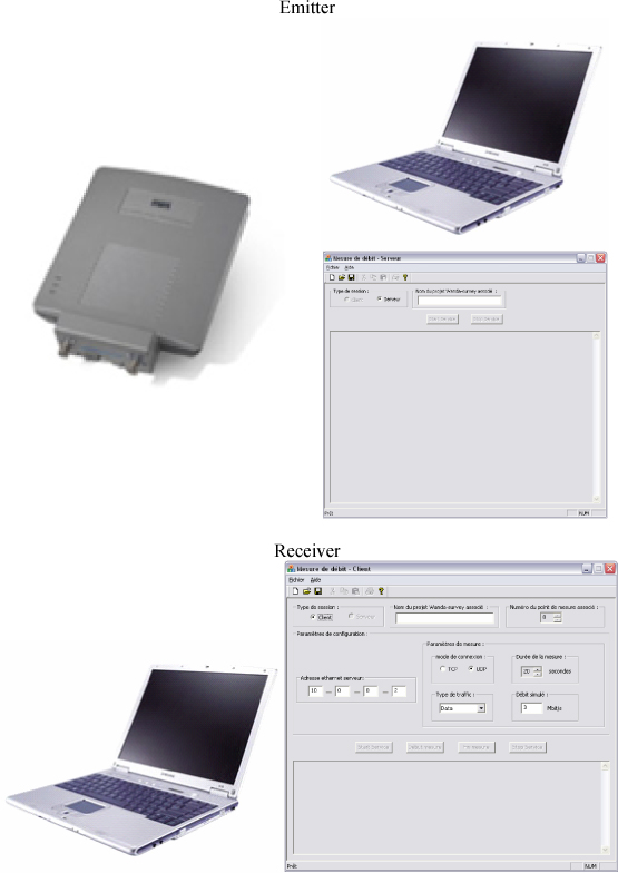
Based on Client-Server architecture, the experimental set-up allows measuring electrical field strength and data rate between a WiFi Access Point driven by a microcomputer (Server) and a measurement laptop system (Client).
The Server, using IPERF software, generates a down link traffic depending on the application:
VOICE: 200 bytes burst
DATA: 550 bytes burst,
VIDEO: 1,350 bytes burst.
The Client (measurement laptop system) records electrical field strength and data rate for each of the application defined above (voice, data, video) on each Server programmed frequency:
2.4 GHz (WiFi 802.11 b/g)
5.2 GHz (WiFi 802.11 a)
The Access Point (AP) emits a power of 20 dBm (100 mW) at 2.4 GHz (WiFi 802.11 b/g) and a power of 23 dBm (200 mW) at 5 GHz (WiFi 802.11 a) respectively. As an illustration we present measurements observed in a three level single family home (BERLIOZ site) on a VIDEO-type downlink traffic between an AP located on the first floor and a client user located on the ground floor.
Measurement equipments consist of CISCO AP (802.11 ab/g) and a PCMCIA WiFi CISCO card (802.11 ab/g). Measurements were performed using AirMagnetTM software associated with the IPERF™ tool for data rate measurements. Data acquisition was performed using the measurement tools developed by France telecom R&D (Tahri et al., 2005). Measurements were taken in a no-interference environment providing optimal data rate values.
Figure 8.8. Schematic representation of the measurement setup
8.5.2. “Berlioz” site
“Berlioz” site is a three levels single-family home, environment where measurements were performed (electric field strength, data rate) (Figure 8.9a):
– basement floor with a garage, a cellar and a laundry;
– ground floor with a kitchen, a living room, a dining room, a bathroom, etc. (Figure 8.9b);
– the first floor with 3 bedrooms, a bathroom, etc. (Figure 8.9b).
Figure 8.9a. 3D representation of the “Berlioz” site
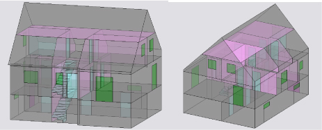
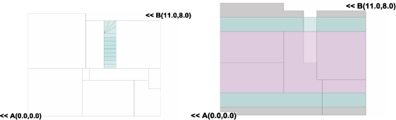
Figure 8.9b. 2D representation of the different rooms in the ground and first floors
8.5.3. Electrical field strength measurements
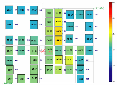
Figure 8.10 gives, as an example, the observed power distribution (dBm) in the ground floor of the “Berlioz” site in different places represented by a colored rectangle (the color is a function of the received power). The access point denoted by a star is placed at 1.75m height above the first floor level. The reader refers to the shaded bar to know the received power (approximate power ranges are marked within boxes). Note that the greater the distance from the emitter and the number of transmitted walls are, the smaller the received power is.
Figure 8.10. Power repartition at 2.4 GHz (WiFi 802.11 b/g) in the ground floor, AP is located in the first floor (Berlioz site)
8.5.4. Data rate measurements
Figure 8.11 shows an example of measured data rate (Mbits/s) in VIDEO context versus received power. Each circle defines a measurement value: average data rate value (Mbits/s) measured as a function of the received power (dBm). All measurements split on the three levels of the house (first, ground and basement floor).
The center curve represents the median evolution of the data rate versus the electrical field strength. It is defined by the following equation:
![]()
where C is the received electrical field strength value
The outer curves define the 90% confidence interval: 90% of the measurements are included between the two curves.
Figure 8.11. Evolution of measured data rates (Mbits/s) in VIDEO context versus the received power at 2.4 GHz (Berlioz site)
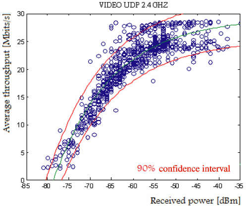
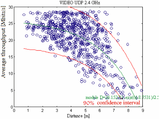
Figure 8.12 shows an example of the evolution of the data rate versus the distance between the emitter and the receiver.
Each circle defines a measurement value: data rate mean value (Mbits/s) measured in function of the distance between the emitter and the receiver (m). All measurements are split on the three levels of the house (first, ground and basement floors).
The center curve represents the median evolution of the data rate versus the distance. It is defined by the following equation:
![]()
where d is the distance between the emitter and the receiver.
The outer curves define the 90% confidence interval: 90% of the measurements are included between the two curves.
Figure 8.12. Evolution of measured data rates (Mbits/s) in VIDEO context versus the distance at 2.4 GHz (Berlioz site)
8.6. Conclusion
We presented, in a radio mobile context, the different measurement methods of electromagnetic waves propagation (field strength in narrow band, impulse response in broad band, angles of arrival and data rates in home environments). The choice of the method depends on environment, frequency band and acquisition speed constraints. Such measurements found, more particularly, applications for the characterization of the different propagation channels in establishing propagation models. Such models are implemented in engineering tools in order to define, design and set up radio mobile communications systems (GSM, UMTS, LMDS, WiFi, WIMAX, etc.).
Field strength measurements in narrow band consist of acquiring at the receiver, at fixed distances intervals, the instantaneous field received from an emitter emitting a fixed frequency continuous signal. Proportional to the electrical field envelope, these measurements reproduce the different variations which affect the signal. A numerical treatment associated with a geographical data base allows us to extract slow variations of great (due to distance), medium scale (due to mask effects) and quick variations (Rayleigh fading).
The methods used for measuring the impulse response of a system can be classified into two families: temporal and frequency methods. Temporal methods regroup impulse emission, correlation of the received sequence with an image of the emitted sequence and Wiener inversion technique. Frequency methods measure the path loss in a given frequency band by performing a frequency scan (vector network analyzers, chirp sounders). The impulse response is then obtained by Fourier transforms. Frequency methods are more specifically adapted to the characterization of the propagation channel more particularly in Ultra Wide Band.
As an example of measuring devices, the main features of the propagation channel sounder AMERRIC defined and developed at France Telecom R&D at Belfort are briefly described. It can be used in particular for obtaining a precise characterization of the radio propagation channel over a bandwidth ranging from 0 to 250 MHz around a carrier frequency ranging from 1.9 to 60 GHz.
DOA are initially determined by simultaneously measuring the impulse response on a multi-sensor array antenna (a linear array antenna) and by comparing the phase evolution for each sensor. Actually, a very directive rotating arm device is associated with the channel sounder receiver. Measurements are performed at constant angular step. A treatment of all measurements allows us to determine a spatial-temporal representation of the impulse response in different geographical configurations (angular power profile, temporal power profile, average spatial-temporal power distribution).
Different methods for determining DOA have been exposed: linear and high resolution methods. Linear methods are based on the Fourier analysis associated with a Wiener inversion or a phase reconstruction. High resolution methods enable a more accurate estimation of the parameters associated with the different multiple paths of a radio propagation channel (amplitude, delay, DOA, etc.) than the traditional linear methods. The MUSIC method is more particularly developed.
Based on Client-Server architecture, electrical field strength and data rates measurements, in the home environment, between a WiFi Access Point and a measurement laptop system have been presented (electrical field strength spatial repartition, data rates in function of the electrical field and the distance between the emitter and the receiver). Such measurements find more specific applications in the deployment of WiFi networks.
8.7. Glossary
| AMERICC | Impulse response measurement system for radio channel characterization |
| CB | Coherence Band |
| BPSK | Binary Phase Shift Keying |
| ESPRIT | Estimation of Signal Parameter via Rotational Invariance Techniques |
| FOSS | Forward Only Spatial Smoothing |
| FTR | amp;D/RESA/NET France Télécom/réseaux d'accès/Network Engineering Tools |
| GPS | Global Positioning System |
| HIPERLAN | High PERformance radio Local Area Network |
| IPERF | Measurement tool for measuring maximum TCP and UDP bandwidth performance |
| LMDS | Local Multipoint Distribution Service |
| MISO | Multiple Input Single Output |
| MIMO | Multiple Input Multiple Output |
| MUSIC | MUltiple SIgnal Classification |
| PRS | Pseudo Random Sequences |
| SAGE | Space Alternating Generalized maximization Expectation |
| SDMA | Spatial Division Multiple Access |
| SIMO | Single Input Multiple Output |
| SISO | Single Input Single Output |
| ULB | Ultra Large Band |
| UWB | Ultra Wide Band |
| UMTS | Universal Mobile Telecommunication System |
| WiFi | Wireless Fidelity |
| WIMAX | Worldwide Interoperability for Microwave Access |
8.8. Acknowledgments
The author would like to thank P. Pajusco, J.Y. Thiriet, J.M. Conrat, V. Guillet, S. Durieux, A. Averous, N. Malhouroux, C. Moroni, L. Cartier of FTR&D, Belfort for their works in this field and P. de Fornel for his help with the translation.
8.9. Bibliography
Barbot J.P., Levy A.J., “Indoor wideband measurements at 2.2 GHz in a shopping center”, PIMRC ‘93 Conference, Yokohama, Japan, 1993.
Balanis C.A., Antenna Theory: Analysis and Design, Arizona State University, 1990.
Conrat J.M., Thiriet J.Y, Pajusco P., l'outil de mesure du canal large bande radioélectrique développé par France Télécom R&D, 4ièmes journées d'études Propagation électromagnétique dans l'atmosphère du décamétrique à l'angström, Rennes, AMERICC, 2002.
Cosquer R, “Conception d'un sondeur de canal MIMO – Caractérisation du canal de propagation d'un point de vue directionnel et doublement directionnel”, IETR, Rennes, 2004.
COST231, “Evolution of land mobile radio (including personal) communications”, Final Report, Information, technologies and Sciences, European Commission, 1999.
Electrobit, http://www.elektrobit.com/index.php?209, 2009.
Ertel R.B., Cardieri P., Sowerby K.W., Rappaport T.S., Reed J.H., Overview of spatial channels for antenna array communications systems, IEEE Personal Communications, February 1998.
Fuhl J., Molisch A.F., Bonek E., “A new single snapshot algorithm for direction of arrival (DAO) estimation of coherent signals”, Special issue on signal separation and interference cancellation for PIRMRC, 1993.
Guisnet B., Verolleman Y., “Evaluation of different methods of directions of arrival using a circular array applied to indoor environments”, Vehicular Technology Conference, Atlanta, Georgia, USA, 1996.
Guisnet B., Perreau X., “Validation of an accurate Direction Of Arrival measurement set-up and experimental exploitation”, 3rd European Personal Mobile Communications Conference, Paris, 9–11 March 1999.
IPERF, http://www.openmaniak.com/fr/iperf.php, 21 August 2009.
Jimenez J., “CODIT Propagation activities and simulation models”, Proc. RACE MPLA Worshop, p.673–677, Amsterdam, May 1994.
Kauschke U., “Wideband indoor channel measurements for DECT transmitter positioned inside and outside office building”, Proc. PIMRC'94 and WIN, vol. IV, p.1070–1074, The Hague, 1994.
Klein A., Mohr W., Thomas R., Weber P., Wirth B., “Direction of arrival of partial waves in wideband mobile radio channels for intelligent antenna concepts”, Vehicular Technology Conference, Atlanta, Georgia, 1996.
Lähteenmäki J., “Determination of dominant signal paths for indoor radio channel at 1.7 GHz”, PIMRC ‘93 Conference, Yokohama, 1993.
Laspougeas P., Pajusco P., Bic J.C., “Radio propagation in urban small cells environment at 2 GHz: Experimental spatio-temporal characterization and spatial wideband channel model”, Proc. IEEE Vehicular Technology Conference (VTC '2000), Boston, 2000.
Lee W.C.Y., Mobile Communications Engineering, McGraw-Hill, New-York, 1986.
Levy A.J., Rossi J.P., Barbot J.P., Martin J., “An improved sounding technique applied to wideband mobile 900 MHz propagation measurements”, Proc. 40th IEEE Vehicular Technology Conference, Orlando, USA, 1990.
LST, http://www.hyper-rf.com/Hyperfrequences/Technologies/Notes-Applications/Sondeur/sondeur-2-G2RM.html, 2004.
Medav, http://www.channelsounder.de/purspec.html, 2009.
Nawrocki A., Contribution à la modélisation des câbles monotorons par éléments finis, PhD Thesis, Nantes University, 1997.
Pagani P., Tchoffo Talom F, Pajusco P., Uguen B., Ultra Wide Band Radio Propagation Channel, Iste, John Wiley & Sons, 2008.
Pajusco P., “Experimental characterisation of directions of arrival at the station in rural and urban area”, Vehicular Technology Conference, Ottawa, Ontario, Canada, 18–21 May 1998.
Parsons J.D., The Mobile Radio Propagation Channel, Pentech Press Publishers, 1992.
Pastel, http://pastel.paristech.org/2667, 2006.
Rossi J.P., Barbot J.P., Levy A.J., “Theory and measurement of the angle of arrival and time delay of UHF radiowaves using a ring array”, IEEE Transactions on Antennas an Propagation, vol. 45, no. 5, p.876–884, May 1997.
Scipion, http://www-iono.enst-bretagne.fr/scipion.html, 11 July 2004.
Schmidt R.O., “Multiple signal location and signal parameter estimation”, IEEE Transactions an Antenna and Propagation, vol. 34, no. 3, 1986.
Tahri R.; Guillet V., Thiriet J.Y., Pajusco P., “Measurements and calibration method for WLAN indoor path loss modelling”, 6th IEE International Conference on 3G and Beyond, pp.1–4, 2005.
Tewfik A.H., Hong W., “On the equivalence of uniform circular arrays and uniform linear arrays”, Proc. of Fifth ASSP Worshop on Spect. Est. and Modeling, pp. 139–143, 1990.
Thompson J., Grant P., Mulgrew B., “Smart antenna arrays for CDMA systems”, IEEE Personal Communications, October 1996.
Vu V. Y., Conception et réalisation d'un sondeur de canal multi-capteur utilisant les corrélateurs cinq-ports pour la mesure de propagation à l'intérieur des bâtiments, PhD Thesis, Ecole Nationale Supérieure des Télécommunications, Paris, 2005.
Zayana, Karim (2003) Méthode de mesure et de modélisation de canaux de propagation radiomobile, Doctorat Electronique et communications numériques, ENST - COMELEC Communication et Electronique, ENST, 2003
Zollinger E., “Measured in house radio wave propagation characteristics for wideband communications systems”, 8th European Conference on Electrotechnics, EUROCOM'88, Stocklom, Sweden, p.314–317, 1988.
Zoltowski M.D., Mathews, “Direction finding with uniform circular arrays via phase mode excitation and beamspace root –Music”, ICASSP, 1992.
1 Chapter written by Hervé SIZUN.