
Chapter 12
Long Baseline Decameter Interferometry
between Nançay and LOFAR1
12.1. Introduction
LOFAR (LOw Frequency ARray) is a very large array of low frequency (LF) antennas, currently under construction in the Netherlands (www.lofar.org). LOFRA is an interferometer in which each antenna is actually a phased array of elementary antennas (crossed dipoles), called “stations”. In its original version, LOFAR was made of 77 stations, 32 of which gathered in a compact configuration (“virtual core”), the other 45 providing interferometric baselines up to 100 km from the “virtual core” (the current LOFAR version in construction - LOFAR Phase 1 will consist of about 40, i.e. 20 + 20, stations). The frequency ranges covered by LOFAR are 30–80 MHz and 110–240 MHz, on both sides of the FM band. At these frequencies, 100 km baselines provide an angular resolution of 20″ at 30 MHz and 7″ at 200 MHz (proportional to the wavelength λ).
Many scientific programs could take advantage of a 10 times better resolution, typically of order of an arcsecond. These scientific objectives are described in detail in Vogt (2006). Here we will restrict ourselves to a single example: the fast imaging of LF radiosources in Jupiter's magnetosphere, whose scientific implications, described in (Zarka, 2004), include:
– improved mapping of the surface planetary magnetic field, via imaging of instantaneous cyclotron sources of the highest frequency;
– improved mapping of the Jovian plasma environment (especially the Io torus) via the propagation effects that it induces on the radio waves propagating through it (especially Faraday rotation);
– direct imaging of the electron beams propagating along magnetic field lines, and of the distribution of electric potential drops along Jovian magnetic field lines;
– detailed study of the magnetospheric dynamics via direct measurements of radiosource locations in the magnetosphere (auroras, satellites magnetic footprints);
– detailed study of radio emission mechanisms via measurement of the emission diagram of the corresponding sources.
The extension of LOFAR to baselines in the order of 1,000 km also has the motivation to Europeanize the project. In France, the first step consists of the installation of a LOFAR station in Nançay (www.obs-nancay.fr) that will take place in late 2009.
The terrestrial ionosphere induces propagation effects on LF radio waves: refractive (intensity scintillations, time-frequency dispersion of the emissions, random motions and focussing/defocussing of source images) and diffractive (scintillations, temporal, spectral and spatial broadening of sources). These effects become stronger at lower frequencies.
The intensity of these effects varies in λn with n typically ~2 (1 to 4). In particular, random time-variable phase fluctuations are introduced by the ionosphere. When the distance between two observation points increases, the correlation between these phase fluctuations decreases. This causes a progressive loss of the mutual coherency of the wave packets received at these two points, canceling their cross-correlation, and thus making (phase) interferometry impossible.
The isoplanetic patch in the ionosphere is in the order of 20 km, which corresponds to the typical horizontal scale of travelling ionospheric disturbances (TIDs) (Mercier, 1989), and it is believed that the coherency of received waves is preserved for baselines up to 100 km (Noordam, 2004). This is not necessarilly true for baselines of 1,000 km.
The question addressed here is: what fraction of the time is the phase coherency of LF waves, received at ~1,000 km, separation preserved (and thus permits interferometric measurements), and is this as a function of time and frequency? Several LF interferometry experiments have been carried out since 1965, at frequencies as low as 18 MHz and baselines up to 7,000 km. We can cite the following studies:
– Jupiter at 34 MHz (in a narrow band: δf = 3 kHz), with a baseline of 4,300 km (Dulk, 1970);
– Jupiter at 18 MHz (δf = 2.1 kHz), with baselines of 218 to 6,980 km (Brown et al., 1968; Lynch et al., 1976);
– 4 radiosources of the 3C catalog at 81.5 MHz with baselines ≤ 1,500 km (Hartas et al., 1983);
– the Crab radiosource at 20 and 25 MHz with a baseline of 900 km (Megn et al., 1997).
However, these studies remained isolated or limited. All were performed within narrow frequency bands, using 1-bit digitization of the waveform down-converted to the baseband by heterodyne reception before correlation.
In 2004, we thus proposed to perform (V)LBI ((very) long baseline interferometric) observations at LF between the Nançayb decameter array (NDA) and LOFAR's initial test station (ITS) in Exloo (NL), separated by 700 km.
12.2. Observations
The observations were performed with a very broad band (40 MHz), digitized directly in the baseband (at 80 MHz rate) with 12 to 14 bits, which provides a large dynamic range, with a real long baseline (Exloo-Nançay) of the future extended LOFAR network. The target of these observations had to be intense (due to the relatively low sensitivity of the instruments used, whose effective areas are a few thousand m2), and much smaller than the fringe width that corresponds to a baseline of 700 km, in order to observe interference fringes. Jupiter fulfills these two conditions in the decameter range, but its emission is sporadic and only partly predictable (Genova et al., 1989).
Jupiter's magnetospheric radio emissions (Zarka, 1998) consist of slowly variable components (at a timescale of several minutes) and brief bursts (a few to a few tens of milliseconds). They are very intense (105–6 Jy; 1 Jy = 1 Jansky = 10−26 Wm−2Hz−1), have frequencies below 40 MHz, and display an elliptical polarization (righthand elliptical polarization dominates the radiation detected from the Earth). The occurrence of the most intense components (which include the bursts) depends on the geometry Io-Jupiter-observer (Figure 12.1).
The radiation pattern of the emissions is very anisotropic, with emitted radiation concentrated along the walls of widely open cones, whose axis is along the magnetic field vector in the source. Previous VLBI observations (Dulk, 1970) led to a conclusion that, assuming an incoherent source, its instantaneous size should be < 400 km at Jupiter, or 0.1″ as seen from Earth.
The instruments used are:
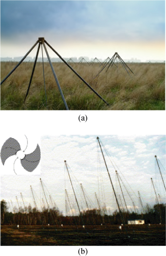
– The LOFAR-ITS station in Exloo (Figure 12.2a), made of 30 “V”-shaped crossed dipoles, whose combination of received signals provides access to the full polarization (4 Stokes parameters) of incident waves. The frequency range covered is 5–35 MHz (well adapted to the observation of Jupiter). The signal from each antenna is digitized on 12 bits at 80 MHz (hence a full coverage of the 0–40 MHz band in baseband). The recorded waveform is stored in the RAM of the acquisition Pcs connected to the antennas. As 1 Go of RAM is available per antenna, it is possible to record 6.7 seconds of continuous waveform from all antennas.
Acquisition must be stopped during the few minutes required for writing the data on disk, and a new 6.7 sec “snapshot” can again be recorded. The phasing of the antennas (“beamforming”), which permits us to synthesize a beam towards a selected radiosource is performed offline: by processing of data blocks of 0.2 sec with Hamming windowing followed by Fourier Transform (FT) of the signal from each antenna, application of a phase gradient equivalent to a time delay to perform the phasing, summation, and inverse FT to get the reconstructed waveform. See Nigl et al. (2007) for more details.
– The NDA (Boischot et al., 1980) in Nançay (Figure 12.2b), is made of spiral antennas with a logarithmic step and wired around a cone, sensitive to the circular polarization of incoming waves, whose combination also gives access to the 4 Stokes parameters. The NDA is composed of 72 left-hand and 72 right-hand polarized antennas. The frequency range covered is 10–100 MHz.
Beamforming is performed in real time via analog antenna phasing, by combination of rotation of elementary antennas (through electronically-controlled switching of antennas wires, by 45° steps) and delay lines between groups of 8 antennas. The signal of the left or right polarized beam can be digitized on 14 bits at 80 MHz (Signatec PDA 14 board – allowing for a full analysis of tha range 0–40 MHz in baseband), and the corresponding waveform can be continuously recorded to disk, limited only by disk capacity (500 Gb permits ~1 h of continuous acquisition).
Figure 12.1. Occurrence probability of Jupiter's radio bursts, as a function of the observer's Jovicentric longitude (called “central meridian longitude”) and the orbital phase of Io counted in the directly from the anti-observer direction. Dotted lines represent the 8 daily hours of observation of Jupiter from Nançay in November 2005 (meridian transit ± 4 h – the transit time is indicated in UT at the center of each daily track, and the corresponding day of the month at the start of each track). Regions noted A, B, C, D approximately delimit intervals of high probability of occurrence of Jupiter's emission (Genova et al., 1989). Hatched areas correspond to occurrence of emissions with frequency >32 MHz. In these areas, occcurrence probability reaches 100%. Such a favourable configuration occcured on November 30. Corresponding observations studied here were recorded within the red segment
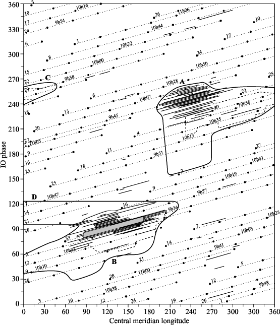
Figure 12.2. (a) LOFAR's Initial Test Station (ITS) made of crossed V-shaped-dipoles. (b) The Nançay decameter array (NDA - insert: a log-spiral conical antenna seen from above, made of 8 conductive wires)
Time references on the two observation sites play a crucial role for VLBI observations. The two instruments used were not originally designed for this type of observation, but the clock stability required at low frequencies is less constraining than at higher frequencies (50 times less at 20 MHz than at 1 GHz). The relative (short-term) time reference was consequently provided to ITS by a crystal synchronizing all acquisition PC, while absolute time was obtained via an Internet time server. At NDA, a GPS clock controlled the periodic insertion – in addition to the sky signal – of the output of a broadband noise generator, during 5 msec per second, starting at every exact absolute second. This intense additional signal is readily visible in the recorded waveform, to the accuracy of a single sample (12.5 nanoseconds), which would not be the case for the signal of a line generator. Note however that the accuracy of GPS time for civil applications is in principle limited to ± 340 nanoseconds, by a deliberate distorsion of the satellite signal, for military security reasons.
An observation session consisted of launching the simultaneous acquisition of waveform snapshots at ITS and NDA, when intense Jovian emission was occurring, with the purpose of cross-correlating them offline. A low resolution (1 spectrum/sec) real time survey of the Jovian radio activity is available only from Nançay (http://www.obs-nancay.fr/a_index.htm + select NDA + real-time display). First attempts, planned using standard probabilities of occurrence of Jupiter's radio emission (Figure 12.1) and a phone line Nançay-Exloo were unsuccessful. The control screen of ITS acquisitions was then exported too the NDA via the Internet, permitting us to launch from Nançay, quasi-simultaneous waveform acquisitions at NDA and ITS, depending on real-time monitoring of Jupiter's activity. Moreover, we found that within the restricted regions of the plane (central meridian longitude, Io phase) where emission reaches or exceeds 32 MHz, the probability of occurrence of Jovian radio emission reaches ~100% (Figure 12.1). We were able to successfully perform simultaneous observations on 30 November 2005. In the following, we describe the complete analysis of a 6.7 sec acquisition snapshot.
12.3. Analysis
“Millisecond” radio bursts (Zarka, 1996) were recorded simultaneously on both sites, mostly in the range 20.7–23.8 MHz. Sample dynamic spectra (intensity versus time and frequency: I(t,f)) are displayed in Figure 12.3. The quasi perfect correspondence between individual bursts seen on the two dynamic spectra is very clear. In addition, horizontal fringes alternately bright and dark appear on ITS data (Figure 12.3a). They consist of Faraday fringes due to the fact that the Jovian radio emission is elliptically polarized and observed by ITS with linearly polarized antennas. Propagation through the Jovian magnetospheric plasma, the interplanetary medium, and the terrestrial ionosphere, causes the rotation of the linear polarization plane of the waves of a frequency-dependent angle θ:
![]()
with X in m, and the rotation measure R = 0.8 ∫L Ne B// dL, with Ne (cm−3) the electron density in the traversed medium, B// (in μG = 0.1 nanoTesla) the magnetic field projected along the ray path, and L the distance in parsecs, or:
![]()
with the dispersion measure [DM] in pc.cm−3, B// in Gauss and f in MHz.
The differential Faraday rotation between two frequencies can be written:
![]()
Intensity maxima are observed at frequencies where the incident wave is aligned with the receiving dipole, and minima at frequencies where the incident wave is orthogonal to it. Faraday fringes do not show up at NDA, because only the right-hand circular component (dominant) of the emission is digitized. Figure 12.4 compares the average spectra (over 6.7 sec) measured by the EW and NS dipoles of ITS to the computation of corresponding Faraday fringes, represented here by |sin(θ(f))| functions. The good fit allowed us to select the centers of bright fringes for cross-correlation with the NDA signal. We note that EW and NS fringes are complementary and that these two signals can be combined in order to synthesize a right-hand circularly polarized waveform.
Figure 12.3. Dynamic spectra of Jupiter “millisecond” radio bursts recorded simultaneously with the NDA (top) and ITS (bottom). The same fine structures are detected. ITS observations in linear polarization are affected by Faraday fringes (horizontal)
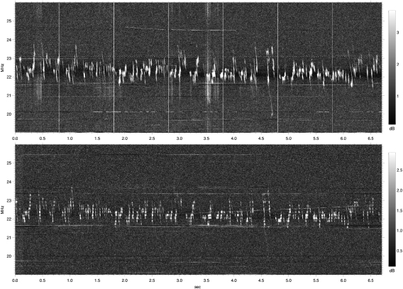
Figure 12.4. Faraday fringes (integrated over 6.7 sec) detected by ITS in EW and NS polarization. A fit in |sin(θ(f))| to fringe positions is superimposed
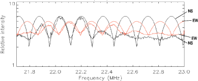
Figure 12.5. Sample dynamic spectra of (a) NDA; (b) ITS. (c) Cross-correlation coefficient of (a) and (b) as a function of time-delay and frequency shift. Cuts of (c) passing by the peak value (d) at zero spectral shift and (e) at time delay ~2.5 msec, which provides the best synchronization
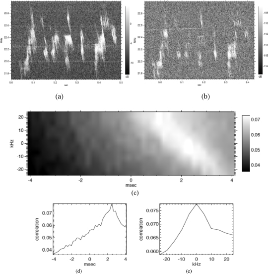
Detection of a significant cross-correlation requires the synchronization of the two recorded waveforms. The absolute temporal accuracy on each of the two waveforms was initially < 1 sec, but >> 12.5 nsec (the sampling step). To increase this accuracy and minimize the computing time for searching the correlation within a defined window, we have first used the Jovian emission as a relative time reference in order to “pre-synchronize” the two data sets, by taking advantage of the presence of sporadic bursts. Dynamic spectra of emissions detected at ITS and NDA have been calculated by sliding-windowed (Hanning) Fourier transform with a spectral resolution δf and a temporal resolution 8t (with the limitation δf × δt ~1). Their cross-correlation C is then calculated as a function of the spectral shift n × δf and time delay p × δt. The maximum of C(n × δf, p × δt) is obtained for n × δf ~0 (as expected for identical baseband digitization at the two observation sites – in fact, a spectral shift of about 190 Hz was measured – discussed below), and a value of p × δt (relative to an arbitrary origin) which determines the synchronization of the two data sets (Figure 12.5). Cross-correlation of dynamic spectra computed successively with an increasing time resolution (an increasingly smaller δt – at the expense of spectral resolution) allowed us to globally synchronize the two data sets with an accuracy of a few microseconds ( < 10 μsec).
We proceeded with waveform cross-correlation within the time window previously determined. This correlation must be computed over a spectral band dominated by the useful Jovian signal, thus much smaller than the initial band 0–40 MHz. Let us recall that previous works were limited to bandwidths of a few kHz. The constraints on the choice of the temporal and spectral window to be used for the correlation and its digital filtering result from: (i) the intrincic time coherency of Jovian radio bursts, consisting of elementary pulses (wave packets) of about 50 μsec duration, and thus of instantaneous bandwidth ~20 (± 15) kHz (Carr et al., 1999); (ii) the presence of Faraday fringes in ITS observations (for each polarization); (iii) digital filtering, which should not significantly increase the time coherency of the signal within the filtered band (which should consequently consist of many frequencies). We have thus selected spectral bands of 100 to 150 kHz width, centered on Faraday fringes maxima (Figure 12.4). Filtering was performed via sliding-windowed FT (215 points Hanning, i.e. δt=0.41 msec >> 50 μsec, and δf = 2.4 kHz < < 20 kHz < 100–150 kHz) of the full band waveform, selection of a [fmin,fmax] band (both frequencies > 0 and < 0, again with Hanning windowing), and FT−1. The waveform in the selcted band is thus reconstructed from the complex spectrum over ~50 frequency channels. Elimination of window edge effects are ensured by a 50% overlap of consecutive 0.41 msec windows, so that we finally retain for each time step (0.41 msec), the central half of the filtered waveform. The filtered and reconstructed waveforms for ITS and NDA are then cross-correlated in the Fourier space (Wiener-Khintchin theorem), as:
![]()
with Wxxx the filtered/reconstructed waveform corresponding to site xxx, and ![]() its variance. We obtain the value of C for τ ∈ [−0.2, +0.2] msec.
its variance. We obtain the value of C for τ ∈ [−0.2, +0.2] msec.
Figure 12.6. Example of synchronized dynamic spectra (a) from NDA and (b) from ITS. The first 2 milliseconds of filtered waveform are displayed below each dynamic spectrum. (c) Cross-correlation of the two 5 msec sample waveforms
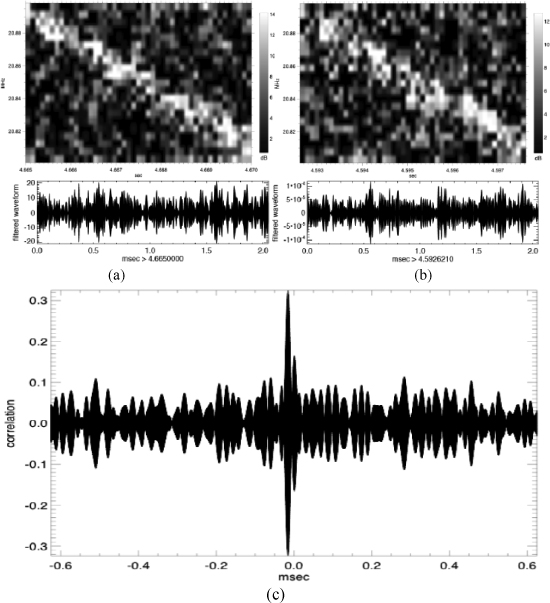
Figure 12.6 illustrates the application of this procedure to a 5 msec x 100 kHz window containing a Jovian burst drifting across the window (from high to low frequencies). Fluctuations of C(τ) display a dispersion σC ~0.05, and a peak > 6σC is observed for a time delay of ~17 (xsec. Note that the oscillation of C(τ) at the center frequency of the studied band (20.85 MHz), can be eliminated by summation of the above C(τ) with C(τ+T/4), i.e. the same cross-correlation function obtained after introduction of a quarter of the period (1/20.85 μsec ~12 nsec ~1 sample) shift between the waveforms WNDA and WITS. Another consequence of this operation is an increase of the the correlation S/N ratio, by a factor of √2. We then extended this analysis to a systematic study of our 6.7 sec × 3 MHz data, divided into 20 spectral bands 100 to 150 kHz wide (corresponding to the above Faraday fringes, excluding their minima), and in time windows 2.5 to 1,000 msec wide. Figure 12.7 displays the time-frequency distribution of correlation coefficients obtained for windows of 2.5 and 100 msec. Maximum values of C(τ), which reach 0.7, clearly match intensity maxima in the dynamic spectra of Figure 12.3.
Figure 12.7. Time-frequency distributions of the correlation between NDA and ITS waveforms for a time window of 2.5 msec (top) or 100 msec (bottom). Maximum values indeed correspond to the presence of an intense Jovian signal (see Figure 12.3)
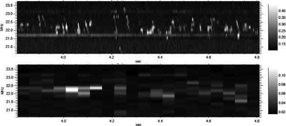
Figure 12.8. Temporal drift of the NDA/ITS time-shift corresponding to a maximum correlation
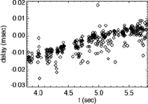
The time shift corresponding to the maximum of C(τ) is determined for each window. It is plotted in Figure 12.8 where only high-correlation points (C(τ) ≥ 0.3) were selected. We observed a systematic drift in this time-shift during the observation, of amplitude ~8.8 μsec/sec (which explains the spectral shift of ~190 Hz noted above). We have looked for the origin of this drift:
– the relative motion of NDA and ITS with respect to the source, due to the Earth's rotation is −177 m/s and −139 m/s respectively; it causes a time drift of ~130 nsec/sec between the two data sets (and a spectral shift of 2.8 Hz);
– the proper motion of Jovian radio bursts source, ~20,000 km/s but in a plane nearly perpendicular to the line of sight (Zarka, 1996), contributes to the drift by about −370 nsec/sec (Nigl et al., 2007);
– time-drifts due to ionospheric and interplanetary propagation are negligible;
– the frequency of the clock controlling waveform acquisition in Nançay was measured using the control signal gated by the GPS time server: the measured sampling frequency is 79,999,998 ± 0.5 Hz, with an associated 1 σ-error of about 1 pixel (12.5 nsec)/sec; the difference from the expected 80 MHz sampling frequency can explain a drift of no more than 100 nsec/sec. Let us recall that the reference provided by the GPS has an associated error of typically 340 nsec, thus the statistical contribution to a drift over 6.7 sec is ~130 nsec.
– finally, it appears that the limited stability of the crystal controlling the PC clocks capturing ITS waveform (~10−5) is the main cause of the observed drift.
12.4. Conclusions and perspectives
The fact that we have obtained high waveform correlations at ~22 MHz confirms the feasibility of interferometric measurements at ~700 km distance even at very low frequencies. This positive results has been obtained until now, only for a sample observation lasting for a few tens of seconds, selected without any a priori knowledge of the ionspheric conditions (in descending phase of the solar activity cycle). No variation of the maximum correlation was measured during the observations. The correlation remains high for time windows ≥ 100 msec and spectral windows ~100 kHz. In contrast with previous studies, we have used a broadband digitization in baseband, with a broad dynamic range. The numerical cross-correlation leaves the time delay between the two waveforms as a free parameter, which allows us to avoid “fringe washing” (the spatial decorrelation effect) due to a fixed delay. Based on the cross-correlation coefficient C(τ), we can derive the visibility V, which characterizes the maximum angular extent of the source (Phillips et al., 1988):
![]()
where the factor √2 corrects for the maximum value (1/√2) of the cross-correlation that can be obtained with one measurement in circular polarization, and one in linear polarization. k is an instrumental factor (close to 1 in our case), and Gτ is the fringe washing coefficient (here = 1), and Si and Ni are the signal (Jupiter) and background noise (galactic) intensities in the two data sets. Our results are consistent with V = 1, an unresolved source as was expected for an observation of Jupiter with an angular resolution of 4″ (700 km baseline at a frequency ~22 MHz).
Figure 12.9. Contribution of the Nançay LOFAR station to the instantaneous coverage of the (u, v) plane (circled in red) by the european extended LOFAR (The Netherlands, Germany, UK and Nançay), at 150 MHz for a source at 80°declination
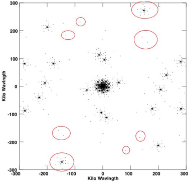
The above analysis can be improved via the synthesis of a right hand polarization signal from the two linear polarizations, recorded at ITS prior to cross-correlamtion with NDA data. More importantly, this observation must be repeated many times in order to quantify the level of correlation that can be reached as a function of time and frequency. As the LOFAR ITS station is no longer operational, we have continued these observations using the NDA and the LOFAR CS-1 (1st station of LOFAR's core) station. This will be pursued with new stations as they are built (e.g. the station in Effelsberg, new Dutch outer ring stations, and the Nançay station itself – expected for December 2009), until finally the NDA is no longer required for these cross-correlation studies. In addition to Jupiter, it will be interesting to observe weaker but non-sporadic sources (≤103 Jy), such as the supernova remnant Cas A (3″ core) and Tau A (Crab SN, with a core of 1.5″). Once they are confirmed and documented, these results will provide a strong support for the development of long baselines for an extended LOFAR network across Europe (see Figure 12.9).
12.5. Acknowledgements
This work is the result of collaboration with L. Denis (Observatoire de Paris, USN/Station de Radioastronomie, Nançay), A. Nigl and J. Kuijpers (Radboud University, Nijmegen, the Netherlands), H. Falcke and L. Bähren (ASTRON, Dwingeloo, the Netherlands).
12.6. Bibliography
Vogt C. (ed.), A Science Case for an Extended LOFAR, ASTRON, Dwingeloo, the Netherlands, 2006.
Boischot A., Rosolen C., Aubier M. G., Daigne G., Genova F., Leblanc Y., Lecacheux A., de La Noe J., Moller-Pedersen B., “A new high-gain, broad-band, steerable array to study Jovian decametric emission”, Icarus, vol. 43, p. 399–407, 1980.
Brown G. W., Carr T. D. and Block W. F., “Long-baseline interferometry of Jupiter at Mc/sec”, Astronomical Journal, vol. 73, no. 6, 1968.
Carr T. D., Reyes F., “Microstructure of Jovian decametric S bursts”, J. Geophys. Res., vol. 104, p. 25127–25142, 1999.
Dulk G. A., “Characteristics of Jupiter's decametric radio source measured with arc-second resolution”, ApJ, vol. 159, p. 671, 1970.
Genova F., Zarka P., Lecacheux A., “Jupiter decametric radiation”, in M. J. S. Belton, R. A. West and J. Rahe (eds.), Time-variable Phenomena in the Jovian System, NASA SP-494 p. 156–174, 1989.
Hartas J. S., Rees W. G., Scott P. F., Duffett-Smith P. J., “Long-baseline interferometry with a portable antenna at 81.5 MHz”, Mon. Not. R. astr. Soc., vol. 205, p. 625–636, 1983.
Lynch M. A., Carr T. D. and May J., “VLBI measurements of Jovian S bursts”, ApJ, vol. 207, p. 325–328, 1976.
Megn A.V., Braude Ya., Rashkovskij S.L., Sharakin N.K., “Decametre radio interferometer system URAN”, (in Russian), Radio Physics and Radio Astronomy, vol. 2, p. 385, 1997.
Mercier C., Genova F. and Aubier M. G., “Radio observations of atmospheric gravity waves”, Ann. Geophys., vol. 7, p. 195–202, 1989.
Nigl A., Zarka P., Kuijpers J., Falcke H., Bâhren L., Denis L., “VLBI observations of Jupiter with the initial test station of LOFAR and the Nançay decametric array”, Astron. Astrophys., vol. 471, p. 1099–1104, 2007.
Noordam J. E., “LOFAR calibration challenges”, Proceedings of the SPIE, vol. 5489, p. 817–825, Glasgow, UK, 2004.
Phillips J.A., Carr T.D., Jorge Levy, and Wesley Greenman, “18 MHz interferometry of nonIo-C L-bursts”, in H.O. Rucker, S. J. Bauer and B. M. Pedersen (eds.), Planetary Radio Emissions II, Austrain Acad. Press, Vienna, p.77–85, 1988.
Vogt C. (ed.), A Science Case for an Extended LOFAR, ASTRON, Dwingeloo, the Netherlands, 2006.
Zarka, P., “Les sursauts ‘S' de Jupiter”, Images de la Physique 95–96, CNRS, Paris, p. 118–127, May 1996.
Zarka P., “Auroral radio emissions at the outer planets: observations and theories”, J. Geophys. Res., vol. 103, p. 20159–20194, 1998.
Zarka P., “Fast radio imaging of Jupiter's magnetosphere at low frequencies with LOFAR”, Planet, Space Sci., vol. 52, p. 1455–1467, 2004.
1 Chapter written by Philippe ZARKA.