
Chapter 10
Measurement for the Evaluation
of Electromagnetic Compatibility1
10.1. Introduction
The measurement of electromagnetic compatibility (EMC) is a very specific field of electromagnetic measurement. In general, it has two objectives corresponding to the two complementary aspects of electromagnetic compatibility. Firstly, EMC measurement aims to measure the characteristics of electric and electromagnetic signals unintentionally produced by a test device — this is emissivity or emission measurement. In this case, the emissivity level must be limited. Secondly, EMC measurement aims to use this same test device to simulate an electric or electromagnetic disturbance device — this is immunity or sensitivity measurement. In this case, the level of immunity must again lie above the minimum acceptable threshold.
To recreate the coupling phenomena likely to occur during the life of a product requires an extensive combination of resources, environments and test conditions. The first difficulty is therefore to define the precise conditions in which the tests should be conducted in order to cover a very wide range of different scenarios identified by experts. This is obviously a vast subject. As an example, an EMC test can reproduce situations as diverse as an analysis of sensitivity to waveforms representing lightning strikes, electrostatic discharge, specific signals relating to power cable interference, etc.
For brevity, we will concentrate our analysis on two large families of tests using direct coupling with an electromagnetic field — emissivity and radiated immunity testing. Through this analysis, we shall show the various requirements in the measurement of electromagnetic compatibility, including those which are inherent to any physical measurement, i.e. the need to ensure representativity, repeatability and good monitoring of measurement errors. Technical and economic feasibility should, of course, be added to the list. The feasibility issue may sometimes explain the limitations of certain measurement protocols. Certain aspects relating to standards, of which there are many in the field of EMC, meet these various requirements and this point is emphasized in the second section of this paper.
The third section of the paper contains a description of the main test environments used when measuring emissivity and radiated immunity, following on from the general remarks on the measurement of EMC included in the second section. The resources described in the third section are still being intensively used at the present time. However, they have a certain number of limitations, especially in light of probable new measurement of electromagnetic compatibility requirements. These points are more extensively developed in section 10.4. Sections 10.5 and 10.6 focus on two specific measurement techniques to which the EMC community is currently devoting a great deal of time and effort — mode stirring reverberation chambers and near-field measurement techniques. These resources may provide answers to some of the needs expressed in the EMC community and are currently undergoing major developments.
10.2. General aspects of EMC measurement
Before analyzing the resources and principles behind electromagnetic compatibility testing in greater depth, we should remember the main aspects of EMC measurement. It is, first and foremost, part of the design process for electronic equipment and complex systems comprised of several different devices. Generally speaking, the EMC design process reveals the requirements for each element within the system. The overall level of interference in a system has to be controlled by judiciously spreading the design constraints (Tesche et al., 1997). This being the case, one of the fundamental roles of EMC measurement is a posteriori demonstration of compliance with these constraints. Although digital model building is increasingly accurate at the design stage, only measurement can provide definitive proof of the quality of the results. Of course, it is essential for the EMC community to agree on the precise test conditions for such measurements. The result is that EMC measurement has become finely structured and standardized over time.
The limits of the standardization are both geographical and sectoral. The various regions of the world (e.g. the European Union) may each draft different standards or impose different levels of stringency for products circulating within a given geographical area. Moreover, the industrial sectors with the highest level of expertise in EMC have developed various standardization strategies. From a more or less historic point of view, the initial stages of standardization have been closely linked to military electronics, military and civilian aeronautics, the telecom sector and, more recently, the automobile and railways sectors. Then there is, of course, the standardization that might be referred to as “other product based”, i.e. the standards applied to all electrical products marketed in Europe, for example. A European directive that came into force in 1996 imposes a minimum number of “essential” requirements with regard to EMC. The standardization sector is then particularly diffuse. In fact, a new set of recommendations and measurement protocols has been introduced, relating to the measurement of human exposure to electromagnetic fields, in particular, as a result of the development of the mobile phone market. A good overview of this standardization situation is described in Champiot et al. (2003), which is said to be regularly updated, or on the search engines of the various standards authorities: such as IEC (CENELEC), ITU (ETSI), ISO, IEEE, RTCA, ANSI, etc.
An EMC standard (or a set of standards) describes the aim of the test, the test environments, the instrumentation required, the relevant waveforms, the calibration procedures used for test equipment and, finally, the test procedure itself. With regard to the IEC, it is appropriate to highlight the work of the CISPR (Comité international spécial des interferences radioélectriques — Special International Committee on Radio Interference), which has published a set of basic standards, CISPR 16, entitled “Specification for radio disturbance and immunity measurement apparatus and methods”. EMC standards can be obtained directly (but not free of charge) from standards authorities. For a more rapid overview of the methods, refer to the aforementioned work or consult any of the following: Montrose et al. (1999) for a description of general techniques; Rybak et al. (2004) for the automobile sector; and Ben Dhia et al. (2006) for component-related techniques, particularly microprocessors, memories, etc.
The primary aim of EMC measurement is to reproduce, more commonly in a laboratory than in situ, a situation that can be summarized in terms of the following three traditional elements:
– source of interference;
– source coupling;
– observation of the result.
In emissivity measurements, the source is the test device itself and the test assesses its interference on the environment in which it is located. In immunity measurements, the source is the reproduction of a situation external to the apparatus. For example, the source of interference may be equivalent to the interference produced by a direct or indirect lightning strike or generated by a telecommunications transmitter located in the vicinity of the test equipment.
The source of interference may be coupled in various ways, i.e. directly by cables, direct radiation or via gaps in electromagnetic shield, proximity couplings or any combination of several of these. For the purposes of metrology, only two types of experiment will be retained — the propagation of interfering signals on any connected lead cable and microwave propagation.
Emissivity testing requires the use of the appropriate coupling devices on input lead cables or the use of antennas to measure the characteristics of the interfering signals. The signals are observed by using an interference spectrum analyzer, again with standard characteristics.
When carrying out immunity testing, the source is generated by the appropriate signals generator and coupled to the system using similar resources. Observations are based on an analysis of the test device behavior. If the behavior is nominal it is reasonable to deduce that the device is insensitive to interference. Otherwise, any dysfunction is attributable to interference. Observation can consist of the visual observation of a malfunction, for example when performing a given task (in particular, a software application) or the observation of the various measurable parameters (observation of changes in the bit error rate for digital communication systems).
One point common to all measurement configurations is that the test device must be used in a realistic operating mode. This may make it extremely difficult to determine operating configurations. Measurement of electromagnetic compatibility is different to other measurements in that a situation of non-compatibility may be the result of circumstances whose simultaneous occurrence is more or less likely. It is therefore dependent on a specific test device operating configuration and associated with a particular coupling situation.
In the following section, we describe the approaches taken in two main families of tests — emissivity and radiated immunity.
10.3. Emissivity and radiated immunity testing
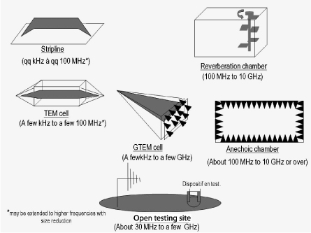
There are many variations in the resources and parameters used to undertake these measurements. This can be partly explained by the diversity of forms and sizes in the objects being tested. For example, a test may be carried out on a component such as a microprocessor, or on a complete vehicle. On the one hand, there is a need to cover a very wide frequency bandwidth, possibly beginning with a kHz (or less) and extending up to 10 GHz or more, depending on the applications.
When considering the resources, a distinction should be made between the test environment and the apparatus required to carry out the tests. The test environment must provide conditions for an electromagnetic field spread that is easy to interpret because it is essential to be able to link observable factors to a known, calibrated characteristic in the electromagnetic field.
Two parameters partly govern the choice of device — the size of the test device and the bandwidth of the device in which its properties are stored. Figure 10.1 gives an overview of commonly-used test environments, depending mainly on bandwidth. Apart from the reverberation chamber, these devices have one major characteristic in common, they deliver a progressive wave with linear polarization. This progressive wave is mostly dissipated in resistive charges: stripline, transverse electromagnetic (TEM) cell and gigahertz TEM (GTEM) cell for the lower section of the bandwidth; or absorbent electromagnetic charges, anechoic chamber and GTEM cell for the upper section of the bandwidth.
In the case of an open site, the absence of any obstacle ensures this type of propagation without the need for any intervention. Because of this, it is possible to establish a direct link between the information observed during generation of the progressive wave. In radiated emissivity, the level of power measured at the output from a cell or at the input to a receiving antenna is directly affected by the source, whose spectrum, polarization and directivity1 can be correctly assessed.
On the other hand, the response from the test device, when solicited by electromagnetic radiation, can be solely attributed to the characteristics of the wave generated as an initial approximation. In fact, the required conditions for simulated propagation in free space are draconian and a tolerance is required. Again, these tolerances are defined by the profession and set down in standards documents. The conformity of a test device is checked during calibration.
Figure 10.1. Various test environments used to measure EMC
10.3.1. TEM and GTEM cells
The TEM cell (Crawford, 1974) provides a very simple means of producing a progressive wave. It acts as a single-mode transmission line. In fact, TEM mode propagation is provided by a transition that adapts impedance between the circular section of the coax cable and the cell and the rectangular section of the cell. The radial lines of the electric field in the coax cable are then polarized vertically between the intermediate metal plate in the cell (septum) and the upper (or lower) wall of the cell. The TEM cell bandwidth is limited by the occurrence of high propagation modes. As a result, the wave formed is no longer uniform. It results from a complex overlay of various modes of propagation in the cell and is difficult to interpret in terms of an analysis of field distribution within the test object. GTEM cells allow for an extension of TEM cells to high frequencies, thanks to the provision of electromagnetic absorbents that act to partly dissipate the non-TEM modes (Crawford et al., 1978). The relationship governing the operation of an ideal TEM cell is as follows:
[10.1] ![]()
where E is the amplitude of the electric field, P is the power transmitted in the cell, Z is the impedance characteristic of the cell and h is the distance between the septum and the upper or lower wall of the cell. The quality of a TEM measurement is assessed mainly by measuring the stationary wave rate at one of the accesses.
Normally, this rate remains low throughout the wavelength used. The field level can also be verified using a local electric field sensor. Calculations show, for example, that the field zone for which the vertically-polarized electric field remains more or less uniform occupies an area centerd between the septum and the upper or lower wall of the cell, with height h/3 and length Lg/3 where Lg is the length of the TEM cell. In this zone, it is also shown that fluctuations in the field around the recommended value are less than 1 dB. Consequently, the TEM cell is an excellent means of calibrating field sensors. In fact, it is very difficult to reproduce such “quiet” field environments in the traditional frequency widths used for radiation analysis by any other means. Any object placed in the cell must be positioned in such as way as to be completely contained within this zone. Likewise, it is possible to generate a wave with reciprocally-controlled amplitude and electric field polarization. The radiation from small devices compared to the wavelength can be compared to the contributions from a basic electrical moment and a basic magnetic moment. The amplitude and direction of these moments can be calculated by creating a vectorial reconstruction of the moments measured, placing the test device in three orthogonal positions (Koepke et al., 1989).
10.3.2. Measurements in an anechoic chamber
The use of an anechoic chamber has long been considered as the only possible means of overcoming the limits of TEM-type guided propagation, especially when carrying out tests in VHF and beyond and/or using larger objects. As regards emissivity, it is the direct radiation from the unintentional source of the device which is analyzed. For immunity, it is the radiation from an external source whose strength is analyzed, once the radiation has been directly coupled to the system. In both cases, the preferred approach is one that minimizes the influence of the environment on the transmission/reception system consisting of the test device or the device generating electromagnetic energy and the test device. In other words, it is necessary to create a propagation channel that is as deterministic as possible, characterized mainly by an attenuation of the radiation in free space, and reducing to a minimum any interference created by the phenomena linked to diffraction or reflection by objects situated nearby.
In this respect there is a solution other than the use of an anechoic chamber. The measurements have to be carried out in an open, obstacle-free space. This is a procedure commonly carried out to measure radiated emissivity only. However, it is not without its drawbacks because measuring the radiation from a test device presupposes that this radiation can be deducted from the radiation pre-existing on the site. Immunity measurements are impossible because the transmission of electromagnetic fields in an open space is prohibited.
An additional question renders the radiated EMC measurement approach even more complex. Is the testing of a device in a highly-idealistic environment such as a fully anechoic chamber really representative of reality? Actually, we are not required to reproduce an environment, which, by definition is completely hypothetical. However, the closer we move towards situations in which propagation in free space is more or less acceptable in various directions above the ground, the more unrealistic it probably is to consider the ground as an electromagnetic absorbent. The radically different hypothesis of a ground represented by a conductive (and therefore perfectly reflective) plane is equally defensible. In fact, it might potentially increase the power of the device as a means of interference.
EMC tests can follow various trends but, in the end, they are based on a consensus. In the following chapters, we set out the main principles for measurement in radiated mode and state our preference among the more recent approaches. As far as radiated immunity is concerned, we will take, as our main reference, standard IEC 61000-4-3, which is widely used and fairly representative of current equipment tests. For radiated emissivity, we will use standards CISPR-22 (CISPR22, 2006) and CISPR 25 (CISPR25, 2006) to describe the main characteristics of the tests. Of course, we do not intend to analyze all the variations; that would be a compilation task without any major benefits.
10.3.3. The main principles behind radiated emissivity testing
Typical radiated emissivity testing layout in an anechoic or semi-anechoic chamber (non-anechoic metal floor) is given in Figures 10.2a and 10.2b. It corresponds to the two steps in the measurement. Stage A is a calibration stage, which is not carried out every time but is done regularly in accordance with the laboratory's quality plan. It consists of checking that the chain of measurements complies with the theory. This conformity is measured taking a level of tolerance set by the standard. Stage B corresponds to the actual measurement and consists merely of placing the test object in the zone occupied by the transmission antenna used for calibration purposes.
There are a certain number of sensitive points in the measurement. It goes without saying that the choice of observation distance D is critical. The measurement zone corresponds to a far-field or near-field zone, possibly in the Rayleigh zone depending on this distance, the frequency bandwidth and the size of the test device. A compromise is usually required because it is impossible to increase D in proportions that would lead to a gigantic chamber (or plot of land for measurements in open spaces). Standard CISPR 22 indicates measurements at a minimum distance of 3 meters, in a frequency ranging from 30 MHz to 1GHz (recently extended to 6 GHz). In this respect, the risk lies more in the high-frequency spectrum of the bandwidth for which the measurement distance may be inadequate if there are sources of radiation located in various zones containing fairly large devices. On the other hand, standard CISPR 25 used in the automobile sector allows for distance measurements of D = 1 m in radio bandwidths, including in long wave (from 150 kHz). Measurement is therefore always carried out in this bandwidth in the Rayleigh zone.
Measurement protocols attempt to detect the maximum interference power of the test device, for each test frequency. This being the case, an object placed on a table or platform can be rotated. The height of the transmission antenna is also adjusted so that the maximum transmission for the given layout can be captured according to standard CISPR 22. The presence of the layout on the ground makes it more than likely that there is an effect on the reception antenna linked to specular reflection via the layout. This contribution is added as a vector to the field radiated directly in the direction of the reception antenna.
Figure 10.2a. Radiated emissivity, Stage A: calibration with vertical polarization
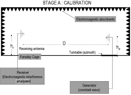
Figure 10.2b. Radiated emissivity, Stage B: test phase with vertical polarization
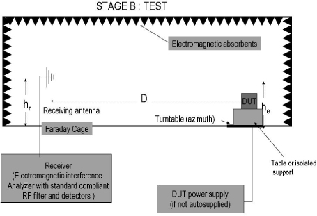
In short, the level of the measured electric field is compared to a template. This presupposes that the characteristics of the receiver are also standardized. Account has to be taken of the diverse nature of the parasite signals measured. They may be produced by periodic narrow-band signals (typically, harmonics from clock signals) or, on the contrary, be bursts with more or less large (temporary) repetition intervals. Thus, the signal filtering and detection technique must be identical in all receivers, in accordance with the definition contained in the standard.
There are of course several weaknesses in this type of measurement, regardless of the current standards. Firstly, the test device is not analyzed in all directions within the space. Azimuth analysis is comprehensive under standard CISPR 22 but elevation is not. This can be explained partly by the fact that there are no economically acceptable means of measuring the complete radiation of a device over a very wide frequency bandwidth. Moreover, it was not deemed necessary to do so in the past because of the low directivity of unintentional radiation. This is generally observed in the lower section of the relevant frequency spectrum. On the other hand, the extension of this type of measurement into higher and higher bandwidths (up to 6 GHz in the 2006 version of CISPR 22) will make this reasoning much less relevant in the future. In the remainder of this chapter, we shall look at the potential in new measurement methods.
Measurement uncertainties are linked mainly to the calibration stage since it can quantify the systematic error committed during measurements in Stage A by direct comparison with the computation. Standard attenuation of the position is determined from knowledge of the characteristics of the antennas used. The basic computation corresponds to an evaluation of the transmission report from two antennas at distance D and at heights he and hr, respectively, above a layout, for various values of the three parameters, based on the dimensions of the equipment being tested. For further information, see Smith et al. (1982). In practice, the tolerances can be as much as +/- 4dB compared to the theoretical values in CISPR 22. This reflects the very real difficulties of using EMC measurements and suggests that improvements may be possible.
10.3.4. The main principles behind radiated immunity testing
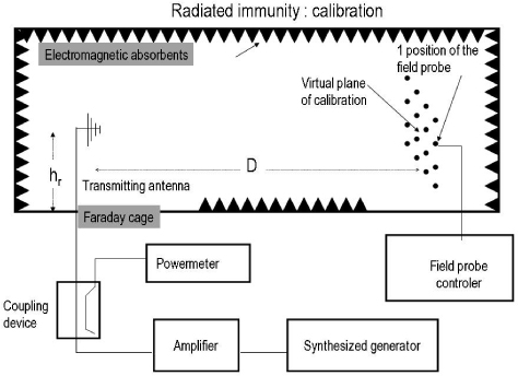
Radiated immunity testing consists of applying a direct radiated field to the test device and testing its reaction to the field. The field characteristic must also be quantifiable. Care must therefore be taken to calibrate the field before beginning the test. There are two calibration techniques, each quite different in principle. The older of the two consists of measuring the field using an electric field probe2 placed close to the illuminated object. The obvious weakness of this technique is the fact that the field measured by the probe is not simply associated with the field transmitted by the transmission antenna but also with the diffraction by the illuminated object. This technique has therefore gradually given way (but has not been totally replaced by) a “substitution” technique in which the test object is not physically present during calibration. The characteristic linking the power transmitted in the field created within the test zone is noted for each test frequency. During the testing of the object, the power is controlled on the basis of the characteristics obtained during calibration, to reach the recommended electric field level required for the test.
Figure 10.3 illustrates the calibration procedure accepted for radiated immunity standard IEC 61000-4-3. The illumination zone is bounded by a square plane, in which the length of the side must be compatible with the maximum size of the test device. The device is placed in such a way that the front of the object coincides with this plane. The test is supposed to be carried out in an anechoic chamber if required by the dimension of the object. In this instance, the electromagnetic radiation is produced by an antenna with linear polarization, located at sufficient distance (typically 3 meters for a 1.5*1.5 meter square) to provide uniform illumination of the square plane. The calibration procedure is therefore identically repeated with horizontal and vertical polarization. The electric field probe is set in 16 positions evenly distributed across the plane. The 16 amplitudes are recorded and the following property is verified for each test frequency:
[10.2] ![]()
where i is the electric field measurement index measured along a rectangular component Er (parallel to the plane, and vertical or horizontal). The test level corresponds to the minimum field level Erc. At this stage, the authorized field fluctuation may appear relatively large. However, these fluctuations are leveled towards the top to ensure that the test level is actually the minimum level to which the test device is subjected. It is, however, obvious that the interpretation of the sensitivity threshold is relatively complex and that the results obtained in the two chambers (calibrated in accordance with the same rules) may be different. The structure presented in [10.2] actually results from a technical and economic compromise, which was deemed acceptable by the scientific community when the standard was being drafted. It is linked, in particular, to the limit on absorbance, especially with regard to specular reflections and the characteristics of the broadband antennas used.
Figure 10.3. Illustration of the calibration stage for a radiated immunity test complying with the IEC 61000-4-3 standard
The object is tested by placing its front in such a way as to coincide with the calibration plane. The test is then carried out on all four sides of the object in succession (no 90° rotation). Note that this type of testing is particularly long. It is carried out on a large bandwidth (typically 256 frequency points between 80 MHz and 1 GHz in accordance with IEC 61000-4-3). It also has to be repeated using both polarizations and the 4 sides of the object. The procedure is further limited in that the top and bottom of the object are not tested. This being so, there is no overall coupling of the object, raising the possible problem, as with radiated emissivity testing, of significant effective coupling sections linked to strong directivity characteristics in the upper spectrum of the test frequencies.
10.4. Efficiency and limitations of EMC measurement techniques
The main merit of the standardized procedures described briefly in the previous section is that they provide the EMC measurement community with a very important benchmark. Test procedures are selected on the basis of theoretical reasoning and technical and economic considerations, which, in the past, have led to choices that can be partly explained by certain approximations or empirical judgments.
Over the past few years, the electromagnetic environment has changed rapidly, raising new questions relating to the sensitivity or emissivity of new generations of devices such as RF transmitter/receivers for new telecommunication services, highrate transmissions on fixed networks, increased frequencies for digital electronics, changes in sensitivity characteristics (low voltage circuits, integration of heterogeneous electronics, etc.). These elements partly change the test as a result of changes in test resources or the production of new resources.
EMC measurement is also subject to major uncertainties. As far as design is concerned, this leads to additional margins in test specifications. Another reason for the greater safety margin is incomplete knowledge of the behavior of the test object, even though it has been subjected to testing. The question of test representativity is therefore an important one. The complexity of the hardware and software configurations of test systems makes the tester's job particularly difficult.
In addition to the support from digital calculation, the opportunity afforded by new test resources to adapt to the current constraints of EMC testing, is currently being considered for many different types of testing, by a research community that is particularly active in Europe. In the next section, we turn our attention to two resources that are particularly likely to provide responses to the changing test techniques used in the field of electromagnetic compatibility.
10.5. Mode-stirred reverberation chambers
In the electromagnetism sector, mode-stirred reverberation chambers first appeared in the 1970s. Initial references suggested the possibility of using reverberation for EMC testing, especially in assessments of total power radiated by structures in the microwave bandwidth (Corona, 1976). This concept had actually already been used for several decades in the field of acoustics. The potential of these chambers was studied in the 1980s in the USA and it was not until the early 1990s that any European scientists began to express an interest in the topic. The chambers are now the subject of many investigations, despite existing standardization. The many advantages of reverberation for use in testing and its efficacy and actual use, however, continue to raise many questions. The concept of reverberation is gradually making massive strides as an additional, useful tool, especially in the evaluation of total radiated power and the radiated immunity of equipment. Its use has also extended to new applications, particularly in the measurement of antennas. In fact, the reverberation chamber is a multi-usage tool that has significantly modified the electromagnetic measurement sector in EMC and radiofrequency (RF) and this trend is expected to continue into the future.
Reverberation techniques have very useful advantages for the measurement of electromagnetic compatibility and a few essential aspects deserve to be highlighted. The results of electromagnetic testing do not depend on the position or direction of the object placed in a reverberation chamber (setting aside statistical uncertainty). If the transmitted power is identical, the mean level of field generated in a reverberation chamber is much higher than in an anechoic chamber and this is crucial given the tendency to increase test levels and given the costs of broadband power amplification. This test resource is intrinsically broadband and it also provides a very specific, additional manner of carrying out electromagnetic testing.
10.5.1. The principles of reverberation
Behavior of a type intrinsic to a reverberation chamber can be obtained in a Faraday cage with dimensions that make it appear oversized at an operational frequency. In fact, a slight variation in frequency (even less than 0.1%) considerably modifies the field distribution in the electromagnetic chamber. At a fixed frequency, a very partial change to the conditions at the limits in the chamber is also sufficient to cause considerable change in field distribution. The reverberation technique consists of modifying certain conditions at the limits continuously or in a discontinuous manner to generate a significant number of uncorrelated field distributions. This modification can be obtained using a device known as a “mode stirrer” consisting of rotating metallic components (see Figure 10.4). Changes in the electric field then follow an almost random pattern of behavior. Initially, it can be shown that any component of the electric field follows a distribution close to that of Rayleigh. The model on which this distribution is based (Kostas et al., 1991; Hill, 1998) consists of seeing the electric field at one point in the chamber as the overlay of a spectrum of plane waves with equally probable incidence and polarization. For a rectangular component in the electric field module, this gives the following theoretical distribution:
[10.3] ![]()
where θ is the Rayleigh law parameter and is linked to the mean of the total electric field squared ![]() , i.e. proportional to the power density in the chamber. It is also possible to verify, through an initial approximation, that the electromagnetic field is uniformly distributed, on average, across all three polarizations. Hence, for a given rectangular component:
, i.e. proportional to the power density in the chamber. It is also possible to verify, through an initial approximation, that the electromagnetic field is uniformly distributed, on average, across all three polarizations. Hence, for a given rectangular component:
[10.4] ![]()
Figure 10.4. The IETR's reverberation chamber and its mode stirrer
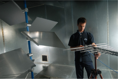
The volume density of energy W is also uniformly distributed in the overall volume V of the chamber. The overall energy stored in the chamber (in a stationary regime) is then Us = WV. This energy is dissipated over time in the walls of the reverberation chamber, or by absorption of the various objects located in the chamber and by the transmission (and possibly reception) antennas. The mean value of the total electric field in the chamber actually depends on the quality coefficient of the chamber Q, defined by convention as:
[10.5] ![]()
where ω is the working impulse and Pd is the power dissipated in the chamber.
The volume density of energy in the chamber is written as:
[10.6] ![]()
The mean of the electric field squared is therefore dependent on the power transmitted Pt, and this power is identical to dissipated power Pd by virtue of the principle of energy conservation given by the equation:
[10.7] ![]()
Consequently, the amplitude of the square of the electric field is directly proportional to the mean quality coefficient of the reverberation chamber. The mean power received by any test object or by an antenna placed in the chamber is also proportional to the quality coefficient. Since no polarization of the field has greater significance than any other, the mean of the total field squared is distributed equally between the three components of the field. The mean of the square of a rectangular field component is therefore ⅓ of expression [10.7]. It is interesting to carry out a rapid comparison of a test environment in an anechoic chamber in which the square of the radiated electric field can be expressed, with a far-field hypothesis, as follows:
[10.8] ![]()
where η0 is the wave impedance of the vacuum, G is the antenna gain and d is the measurement distance. The ratio of the mean of the square of an electric field component in a reverberation chamber (⅓ of [10.7]) to the value of the square of an electric field component in an anechoic chamber [10.8] is therefore:
[10.9] 
The estimation of the quality factor of a reverberation chamber has been the subject of approximate theoretical evaluations (Hill et al., 1994). However, an evaluation in test conditions is absolutely essential to obtain a precise estimation. The quality coefficients of a reverberation chamber can fluctuate significantly depending on the chamber's volume/surface ratio, the material used (copper, galvanized steel, aluminum, etc.), and the various residual leaks or residual absorptions of any materials found in the chamber. Typically, quality coefficients can vary from 103 to 105 for chambers with a size of between 20 and 100 cubic meters, the largest of which operate at between 100 MHz and several GHz. Even if a high-gain antenna is used in an anechoic chamber, the ratio [10.9]3 works to the advantage of reverberation chambers, on a single rectangular field component.
The principle behind electromagnetic measurement in a reverberation chamber is therefore as follows, regardless of the target application. The test object is placed in any position and direction within the useful space of the chamber. The useful space includes all points within the chamber located at a distance equal to at least λ/2 from the object or metallic wall. Below this distance, especially from a metallic wall, the statistical uniformity of the field depending on the three field components cannot be guaranteed because of the conditions at the limits imposed by the wall. This property results from the theoretical model of a plane wave spectrum proposed by (Hill, 1998), from which the spatial correlation properties of the field can be deduced (Hill, 2002). When measuring immunity, the power is adjusted to ensure that the maximum level (i.e. its expectation) of a rectangular component of the recommended electric field is reached. For further details, see (IEC 61000-4-21, 2003).
It is with reference to this maximum level that a test object is presumed to be immune or, on the contrary, sensitive. This is, of course, not without posing a problem with regard to the specification of the level of testing, a point to which we will return in the following paragraph. When measuring emissivity, it is first necessary to determine the insertion losses in the chamber. From this, it is then possible to directly deduce the total power radiated by an object placed in the chamber, the measurement of mean power received by a reception antenna and information on insertion losses. During the test, a check should also be carried out to ensure that the test object has not significantly affected insertion losses (change to the overall quality factor) in the chamber. If it has, the insertion losses should be measured while the object is still present.
10.5.2. Tests in an anechoic chamber and in a reverberation chamber
With regards to the electromagnetic environment, tests in a reverberation chamber are totally different to tests in an anechoic chamber. The solicitation of the test object is therefore different and it is particularly important to lay down a few operating rules, especially in terms of standardization. Reverberating chambers have a wide range of advantages but there is a major difficulty in linking tests in a reverberation chamber to the more conventional tests carried out in an anechoic chamber. This complex subject is currently undergoing investigation, mainly with respect to measurements of radiated immunity. Illumination in an anechoic chamber is a sequence of waves polarized horizontally or vertically along different angles of incidence at the azimuth. Illumination in a reverberation chamber is an overlay of states that solicit the test object in incidence and polarization for a randomly distributed field, as shown in equation [10.3] for Er.
To obtain an idea of the test object's behavior when placed in such widely-differing situations, we have to put forward a number of prior hypotheses even if there is a risk, in doing so, of restricting the applications. Firstly, we consider that the equipment is sensitive to a maximum level of coupling. We then assume that an unintentionally radiating device is rarely sensitive to more than one polarization of the field. In this case, it might be worthwhile adjusting the test level in a reverberation chamber so that the ratio of equation [10.9] is equal to 1. Crossing a critical amplitude threshold for a rectangular field component depends directly on the level of testing in an anechoic chamber (to within the calibration uncertainty which is fairly significant). However, this critical value will almost certainly be reached in a reverberation chamber.
In an anechoic chamber, the fault would be noted when:
[10.10] ![]()
In a reverberation chamber, the fault would be noted with the probability:
[10.11] ![]()
The detection of malfunction in a reverberation chamber is therefore linked to the statistical distribution of the maximum electric field in the chamber. This is the criterion currently retained in EMC standardization and, therefore, the calibration of reverberation chambers is based on an estimate of the maximum field. Knowing the distribution of this maximum is a major criterion for the appreciation of test results from a reverberation chamber and is a significant criterion for analysis of test stringency. It again raises the question of the real distribution of the field within the chamber and the nature of the interaction with the test object. Prudence is required when analyzing test objects with very directive radiation because the reverberating chamber suppresses the directivity observable with illumination by a plane wave in an anechoic chamber. This might justify the increased level in a reverberation chamber.
Major issues have also been raised regarding the statistics estimated from measurements in a real reverberation chamber (Lemoine et al., 2007a) (compared to theoretical statistics resulting from models based on a hypothetical, ideal chamber). These statistics impact directly on the evaluation of the distribution of the maximum field (Orjubin, 2007). The same applies to the important question of the correlation of measurement samples, especially when using reverberation chambers and low frequencies (Lemoine et al., 2007b). A mode stirrer with a rotation axis usually provides the stochastic behavior of the field. It is therefore useful to know the equivalent number of samples independent of the sequence measured over one rotation of the stirrer. This estimation involves a definition of the intrinsic performance of a stirrer depending, for example, on its geometry. It also involves the uncertainty of the measurement and, therefore, maximization of the measurement itself.
10.5.3. Recent and future applications for reverberation chambers
The field of application of reverberation chambers has recently undergone major change, with various applications meeting new needs in electromagnetic compatibility and in the measurement of performance of specific antennas.
As far as EMC measurement is concerned, needs initially related to measurements of radiated immunity and the EMC research community has worked extensively on this topic. Applications relating to the measurement of shield effectiveness have also undergone recent developments (Holloway et al., 2003). This test environment is also very useful for the measurement of radiated emissivity. If there is a source of radiation with total radiated power Pt, a reception antenna in the reverberation chamber will sample reception power such that:
[10.12] ![]()
where < > refers to the empirical estimation of a mean. This gives a mean power (over one rotation of the stirrer) that is approximately proportional to the total radiated power of the object. An evaluation of this power presupposes prior knowledge of the overall quality coefficient for the chamber and this may depend on the object itself dissipating a fraction of its own radiation. The calibration procedure must, of course, take this factor into account, especially when large objects are being tested.
Measurements of total radiated power by an unintentionally-radiating device usually requires a modest degree of precision — only a few dozen samples (of stirrer positions) are required to ensure a statistical uncertainty that is compatible with the requirements of the EMC designer.
Extensions to include the measurement of antennas usually require much greater precision, which means, according to the central limit theorem, a much greater collection of samples. This is actually accessible when using high frequencies in the reverberation chamber, usually thanks to a combination of mechanical and frequency stirring. Frequency stirring is achieved by a modification (possibly step-by-step) limited to a working frequency excursion of the order of 1% in the bandwidth of the antenna. The multiplying effect obtained (Nm samples by mechanical stirring and Nf p by electronic stirring potentially give a total of Nm Nf ) makes a reverberation chamber a very attractive proposition for efficiency measurements (Rosengren, 2001) or measurements of diversity gains in antennas (Kildal, 2002). The main advantage of a reverberation chamber for this type of assessment is the independent positioning of the antenna and the opportunity to test the antenna in various environments given the very large number of tests available. Very recently, researchers began to consider the use of reverberation chambers to emulate standardized propagation channels when testing communication systems (Holloway, 2006).
10.6. Electromagnetic near-field measurement techniques applied to EMC
10.6.1. Near-field techniques in a Rayleigh zone
Electromagnetic near-field measurements have been in use for a very long time but the corresponding methods and objectives have undergone considerable development. The use of electric or magnetic field sensors quickly became commonplace, initially with a view to detecting zones that were very active with regards to electromagnetic radiation. It is possible to locate these zones using basic sensors that are easy to build. By moving them all around the equipment (or across a predetermined surface), it is possible to assess radiation. These highly qualitative procedures tend to be used before or after more quantitative standardized measurements in far-field zones (or at least in a non-reactive zone) to measure the integral radiation of the device. Qualitative near-field measurements are used to locate zones that may be responsible for the possible excess radiation identified in a far-field before a solution to the radiation is implemented. Many electromagnetic compatibility laboratories are therefore equipped with sensors (magnetic loops or basic electric dipoles) for this type of diagnosis and they issue design recommendations on the subject.
However, over the past decade or more, near-field measurements have undergone major changes, in response to a number of objectives. Firstly, there was a need to refine near-field measurements as a diagnostic tool, especially to measure radiation from printed circuit boards or measure integrated components. Such components are playing an increasingly critical role in radiated emissivity, as they constitute the main sources of radiation. Test analysis will also affect design. As an example, a microprocessor, which includes a large number of transistors, produces intense activity linked to the consumption of electricity during switching phases. As such, it is very important to detail its behavior so that the design of the microprocessor and the integrated circuit can be modified (Ben Dhia et al., 2006).
Testers began by manually manipulating sensors but this led to the design of automated systems for the measurement of a defined surface at a standard distance from the test object. There are many strategies based on this system, most of them the results of compromise. Initially, it is the spatial resolution of the field map that will guide the choice of measuring distance and the design of the measuring sensors. The size of the probe partly conditions the spatial resolution of the measurement. Its actual area of coupling with the field increases with its size, however, leads to a lower spatial resolution. The sensor also has a greater effect on the electromagnetic behavior of the test object. Inversely, the use of very small sensors limits measurement perturbation but these small probes are much less sensitive and the measurements take longer to complete. Measurement distance is another essential parameter. Accessibility of the spatial distribution of radiation sources increases as the measurement distance decreases. Naturally, decreasing the measurement distance increases the risk of the test device and probe mutually affecting each other.
In addition to monitoring the profile of the measurement height above non-plane surfaces, it is also necessary to deconvolute the response from the sensor to obtain the electromagnetic radiation actually produced by the probe. This requires a number of calibration procedures, using test devices with known radiation characteristics. For example, analysis can be carried out on the radiation from a board including a micro-stripline powered by a frequency-synthesized generator. The development of various field sensor types (Gao et al., 1996, 1998; Slattery et al., 1999) has led, in turn, to the development of highly efficient test beds.
10.6.2. Near-field techniques outside the Rayleigh zone
Stratton (1941) published the theoretical foundations for the expansion of the electromagnetic field within various markers based on knowledge of the conditions at the limits. Knowledge of the electromagnetic field sampled on a closed surface surrounding a source of radiation is sufficient to determine the expression of the electromagnetic field at every point in the space outside the measurement surface. A near-field measurement can therefore be turned into a far-field equivalent. Under certain conditions, when the measurement distance is located in the Fresnel zone, knowledge of the tangential electric field may be sufficient. As far as testing is concerned, it was not until the 1970s that the first near-field measurement methods were developed, in association with the far-field calculations. The following paragraph indicates the general principles behind near-field measurements in a sphere surrounding the radiating element. Taking propagation in free space as a given, within a spherical marker (O,r,θ,φ), the electric field radiated by a source confined to the center of the marker is written as:
[10.13] 
where Qsmn represents the weighting coefficients for the spherical harmonics of degree n and order m, Y0 the wave admittance from the middle of uniform propagation and Fsmn the functions of spherical orthogonal and standardized waves forming the basic vectors of the generic solution of the Helmholtz equation. S is the mode type index (TM or TE). The various functions Fsmn are linked to the corresponding standard Legendre polynomial ![]() of degree n and order m (Hansen, 1988). Sequence [10.13] is infinite but the electromagnetic energy is distributed in a limited number of modes. This limitation is linked solely to the intrinsic dimension of the source of radiation. Thus, if the source is contained within a sphere with radius a, we can consider limit N to be of the order of the spherical harmonics such that:
of degree n and order m (Hansen, 1988). Sequence [10.13] is infinite but the electromagnetic energy is distributed in a limited number of modes. This limitation is linked solely to the intrinsic dimension of the source of radiation. Thus, if the source is contained within a sphere with radius a, we can consider limit N to be of the order of the spherical harmonics such that:
[10.14] ![]()
where e.u.n. refers to the entire upper number and k is the wave number.
Theoretically, it is therefore unnecessary to define an antenna beyond order N, which translates the limit in the spatial variation of the electromagnetic field emitted by a source with finite dimensions (Bucci, 1987). In fact, this remarkable property represents an opportunity to create measurements by displacing a sensor at regular intervals across the elevation and azimuth of an angle.
![]()
In practical terms, several units are added to the order N, to carry out over-sampling and improve the accuracy of the measurement. The coefficients Q are calculated using the orthogonal properties of the functions Fsmn. The calculation takes the form of a double integral in θ and φ that can be reduced to Fourier integrals. It is interesting to note that this technique can be fully adapted to non-spherical surfaces, including non-closed surfaces such as, for example, cylindrical or plane surfaces, on the condition that the effects of spatial truncation are taken into account. The modulated diffusion technique paved the way for the use of multisensor measurements, which also significantly increased the speed of measurement (Mostafavi et al., 1985). This technique consists of modulating the electromagnetic RF field using a low frequency signal and a non-linear component. The diffracted field or, more directly, the signal received by the sensor, is then demodulated by synchronous detection, giving access to the amplitude and phase of the radiated field measured locally by the sensor. A network of successively modulated sensors can be used to very quickly scan a large measurement area.
This type of characterization has several major advantages as far as electromagnetic compatibility is concerned. It provides a comprehensive definition of the radiation (total radiated power, radiation pattern) and, more generally, gives access to the radiated field, which can be calculated at any point in the space. The technique may potentially allow for an evaluation of shield effectiveness or the closely-associated coupling section when considering electromagnetic hardening (Sérafin et al., 1998).
The near-field measurement process could therefore be adapted to the measurement of radiated emissivity. However, it presupposes the measurement of amplitude and electromagnetic field phase. Recently, to overcome this problem, a pseudo-temporal measurement technique was proposed, consisting of analyzing the coherence matrix in a narrow band, between the signals received by the various sensors from a near-field base (Fourestié et al., 2005). A coherence matrix consists of all the convolution products for signals recorded in a narrow band (tangential components of the electric field) over all the sensors in the network. By breaking the coherence matrix down into singular values, it is then possible to assess the number of coherent sources, calculate the near-field radiation on the measurement area and therefore, by expansion, calculate far-field radiation.
A number of obstacles still exist to the alternative use of near-field tests to define the radiated emissivity of equipment. However, it is reasonable to think that the future development of near-field techniques might eventually change this. Moreover, the use of near-field characterization provides much more than a solution to the problem of the qualification of antennas or unintentional radiation in the EMC sector. A modal description of electromagnetic radiation might also provide a model. The construction of fictitious sources of radiation (Serhir et al., 2008) and the location of sources responsible for radiation are other examples of major applications in EMC, in a sector in which electromagnetic measurement is used with increasing frequency to supply models that are useful for digital simulation. It is also agreed that digital simulation itself might shed some useful light on the interpretation of measurement results.
10.7. Conclusions and future prospects
The range of EMC standards offers a significant number of different EMC test methods, covering a wide area of investigation in varied coupling situations. These methods, however, are undergoing constant change in line with new demands resulting from complex electronic systems. At present, specifications include EMC constraints at every level of system development, right down to individual integrated components. The complexity of these systems, their level of integration and the changes in the electromagnetic environment are all driving forces behind the search for a maximization of existing test resources and the development of new measurement techniques. Without claiming to have covered every aspect of this subject, we have briefly outlined a few general principles for the measurement of emissivity and radiated immunity, with an indication of the corresponding test environments.
We then concentrated on two families of test resources that are among those most likely to satisfy technological developments. The first group included reverberation techniques, the second, near-field techniques. These techniques provide an alternative to the already existing tools, such as the test environments briefly described in this book. As such, they must now prove their potential as an addition to the conventional EMC testing procedures. They have a certain commonality, in as much as they lie at the junction of two sectors that are linked but often use different resources, i.e EMC measurement and the evaluation of antenna performance. In the future, EMC measurement will not only be used for validation and certification purposes. It will have a more important role, supplying behavioral models that can be integrated into electromagnetic calculations.
10.8. Bibliography
Ben Dhia S. Ramdani M., Sicard E., Electromagnetic Compatibility of Integrated Circuits, Springer, 2006.
Bucci O.M., Franceschetti G. “On the spatial bandwidth of scattered fields”, IEEE Transactions on Antennas and Propagation, vol. 35, no. 12, p. 1445–1455, December 1987.
IEC 61000-4-3, “Testing and measurement techniques, Radiated, radio-frequency, electromagnetic field immunity test”, Electromagnetic Compatibility International Standard, Part 4-3, 2001.
IEC 61000-4-21, “Testing and measurement techniques, Reverberation chamber test methods”, Electromagnetic Compatibility International Standard, Part 4-21, 2003.
Champiot G. et al., Maîtrise de la CEM, Technologie, Réglementation, Normes, reference tables collection, Dunod, 2003.
CISPR 22, “Information technology equipment. Radio disturbance characteristics: limits and methods of measurement”, 2006.
CISPR 25, “Radio disturbance characteristics for the protection of receivers used on board vehicles, boats, and on devices: Limits and methods of measurement”, 2003.
Corona P., Latmiral G., Paolini E., Piccioli L., “Use of a reverberation enclosure for measurements of radiated power in the microwave range”, IEEE Transactions on Electromagnetic Compatibility, vol. 18, no. 2, p. 54–59, May 1976.
Crawford M.L., “Generation of standard EM fields using TEM transmission cells for EMC measurements”, IEEE Transactions on Electromagnetic Compatibility, vol. 16, no. 4, p. 189–195, November 1974.
Crawford M.L., Workman J.L., Thomas C.L., “Expanding the bandwidth of TEM cells”, IEEE Transactions on Electromagnetic Compatibility, vol. 20, no. 3, p. 368–375, August 1978.
Fourestié B., Bolomey J.C., Sarrebourse T., Altman Z., Wiart J., “Spherical near-field facility for chracterizing random emissions”, IEEE Transactions on Antenna and Propagation, vol. 53, no. 8, p. 2582–2589, August 2005.
Gao Y., Wolff I., “A new miniature magnetic field probe for measuring three-dimensional fields in planar high-frequency circuits”, IEEE Transactions on Microwave Theory and Techniques, vol. 44, no. 6, June 1996, p. 911–918.
Gao Y., Ren Q., Wolff I., “Calibration of electric coaxial near-field probes and applications”, IEEE Transactions on Microwave Theory and Techniques, vol. 46, no. 11, p. 694–702, November 1998.
Hansen J.E., “Spherical near-field antenna measurements”, IEE Electronic Waves Series, Peter Peregrinus, 1988.
Hill D.A., Ta M.A, Ondrejka A.R, Riddle B.F., Crawford M.L., Johnk R.T., “Aperture excitation of electrically large, lossy cavities”, IEEE Transactions on Electromagnetic Compatibility, vol. 36, no. 3, p. 169–178, August 1994.
Hill D.A., “Plane wave integral representation for fields in reverberation chambers”, IEEE Transactions on Electromagnetic Compatibility, vol. 40, no. 3, p. 209–217, August 1998.
Hill D.A., Ladbury J.M., “Spatial-correlation functions of fields and energy density in a reverberation chamber”, IEEE Transactions on Electromagnetic Compatibility, vol. 44, no. 1, p. 95–101, February 2002.
Holloway C.L., Hill D.A., Ladbury J., Koepke G., Garzia R., “Shielding effectiveness measurements of materials using nested reverberation chambers”, IEEE Transactions on Electromagnetic Compatibility, vol. 45, no. 2, p. 350–356, May 2003.
Holloway C.L., Hill D.A., Ladbury J., Wilson P.F., Koepke G., Coder J., “On the use of reverberation chambers to simulate a rician radio environment for the testing of wireless devices”, IEEE Transactions on Antennas and Propagation, vol. 54, no. 11, p. 3167–3177, November 2006.
Koepke G.H., Ma M.T., “Implementation of an automated system for measuring radiated emissions using a TEM cell”, IEEE Transactions on Instrumentation and Measurement, vol. 38, no. 2, p. 473–479, April 1989.
Kostas G.K., Boverie B., “Statistical model for a mode-stirred chamber”, IEEE Transactions on Electromagnetic Compatibility, vol. 33, no. 4, p. 366–370, November 1991.
Kildal P.S., Rosengren K., Byun J., Lee J., “Definition of effective diversity gain and how to measure it in a reverberation chamber”, Microwave Optical Technology Letters, vol. 34, no. 1, p. 56–59, July 2002.
Lemoine C., Besnier P., Drissi M., “Investigation of reverberation chamber measurements through high power goodness of fit tests”, IEEE Transactions on Electromagnetic Compatibility, vol. 49, no. 4, p. 473–479, November 2007a.
Lemoine C., (2), Besnier P., Drissi M., “Advanced method for estimating number of independent samples with stirrer in reverberation chamber”, Electronics Letters, vol. 43, no. 16, p. 861–862, August 2007b.
Montrose M. I., Nakauchi E.M, Testing for EMC Compliance: Approaches and Techniques, Wiley IEEE press, 2004.
Mostafavi M., Bolomey J.C., Picard D., “Far-field accuracy investigation using modulated scattering technique for fast near-field measurements”, IEEE Transactions on Antenna and Propagation, vol. 33, no. 3, p. 279–285, March 1985.
Orjubin G., “Maximum field inside reverberation chamber modeled by the generalized extreme value distribution”, IEEE Transactions on Electromagnetic Compatibility, vol. 49, no. 1, p. 104–113, February 2007.
Rosengren Kent; Kildal Per-Simon, Carlsson C., Carlsson J., “Characterization of Antennas for Mobile and Wireless Terminals in Reverberation Chambers: Improved Accuracy by Platform Stirring”, Microwave and Optical Technology Letters, vol. 30, no. 20, p. 391–397, October 2001.
Rybak T., Steffka M., Automotive Electromagnetic Compatibility, Springer, 2004.
Sérafin D., Lasserre J.L., Bolomey J.C., Cottard G., Garreau P., Lucas F., Therond F., “Spherical near-field facility for microwave coupling assessments in the 100 MHz-6 GHz frequency range”, IEEE Transactions on Electromagnetic Compatibility, vol. 40, no. 3, p. 225–234, August 1998.
Serhir M., Besnier P., Drissi M., “An accurate equivalent behavioral model of antenna radiation using a mode-matching technique based on spherical near-field measurements”, IEEE Transactions on Antenna and Propagation, vol. 56, no. 1, pp. 48–57, 2008.
Slattery K.P., Neal J, Cui W., “Near-field measurements of VLSI devices”, IEEE Transactions on Electromagnetic Compatibility, vol. 41, no. 4, p. 374–384, November 1999.
Smith A.A, German R.F., Pate J.B., “Calculation of site attenuation from antenna factors”, IEEE Transactions on Electromagnetic Compatibility, vol. 24, no. 3, p. 301–316, August 1982.
Stratton J.A., Electromagnetic Theory, McGraw-Hill, 1941.
1 Chapter written by Philippe BESNIER, Christophe LEMOINE and Mohammed SERHIR.
1 The direction of maximum directivity is the parameter that determines the size of the EMC design.
2 The notion of a field probe is different to the notion of an antenna. Unlike an antenna, a field probe has only a low level of efficiency because of its small size compared to the wavelength. It is used mainly as a localized field sensor.
3 This expression refers to the statistical mean of the square of a rectangular component, which is more or less exponential. It is not possible to directly deduce the behaviour of the mean of the component module as it complies with a Rayleigh Law. However, the square root of this expression provides some idea, within a few %.