5 Modulation Methods

Modulation is the process whereby message information is embedded into a radio frequency carrier. Message information can be transmitted in the amplitude, frequency, or phase of the carrier, or a combination thereof, in either analog or digital format. Analog modulation schemes include amplitude modulation (AM) and frequency modulation (FM). Analog modulation schemes are still used today for broadcasting AM/FM radio, but all other communication and broadcast systems now use digital modulation. Digital modulation schemes transmit information using a finite set of waveforms and have a number of advantages over their analog counterparts. Digital modulation is a natural choice for digital sources, for example, computer communications. Source encoding or data compression techniques can reduce the required transmission bandwidth with a controlled amount of signal distortion. Digitally modulated waveforms are also more robust to channel impairments such as delay and Doppler spread, and cochannel and adjacent channel interference. Finally, encryption and multiplexing is easier with digital modulation schemes.

Modulation schemes can be designed to provide power and/or bandwidth efficient communication. In an information theoretic sense, we want to operate close to the Shannon capacity limit of a channel. This generally requires the use of error control coding along with a jointly designed encoder and modulator. However, in this chapter we only consider the modulation schemes by themselves. The bandwidth efficiency of a modulation scheme indicates how much information is transmitted per channel use and is measured in units of bits per second per Hertz of bandwidth (bits/s/Hz). The power efficiency can be measured by the received signal-to-interference-plus-noise ratio (SINR) that is required to achieve reliable communication with specified bandwidth efficiency in the presence of channel impairments such as delay spread and Doppler spread. In general, modulation techniques for spectrally efficient communication systems should have the following properties:

Compact power density spectrum: To minimize the effect of adjacent channel interference, the power radiated into the adjacent band is often limited to be 60–80 dB below that in the desired band. This requires modulation techniques having a power spectrum characterized by a narrow main lobe and fast roll-off of side-lobes.
Robust communication: Reliable communication must be achieved in the presence of delay and Doppler spread, adjacent and cochannel interference, and thermal noise. Modulation schemes that promote good power efficiency in the presence of channel impairments are desirable.
Envelope properties: Portable and mobile devices often employ power-efficient nonlinear (Class-C) power amplifiers to minimize battery drain. However, amplifier nonlinearities will degrade the performance of modulation schemes that transmit information in the amplitude of the carrier and/or have a nonconstant envelope. To obtain suitable performance, such modulation schemes require a less power-efficient linear or linearized power amplifier. Also, spectral shaping is usually performed prior to upconversion and nonlinear amplification. To prevent the regrowth of spectral side lobes during nonlinear amplification, modulation schemes having a relatively constant envelope are desirable.

5.2 Basic Description of Modulated Signals

With any modulation technique, the bandpass signal can be expressed in the form

s (t) = R {s ˜ (t) e j 2 π f c t} (5.1)

$s (t) = ℜ {\tilde{s} (t) e^{j 2 π f_{c} t}} (5.1)$

where s˜(t)=s˜I(t)+js˜Q(t) $\tilde{s} (t) = {\tilde{s}}_{I} (t) + j {\tilde{s}}_{Q} (t)$ is the complex envelope, f_c is the carrier frequency, and ℜ{z} denotes the real part of z. For any digital modulation scheme, the complex envelope can be written in the standard form [1]

s ˜ (t) = A \sum n b (t - n T, x n) (5.2)

$\tilde{s} (t) = A \sum_{n} b (t - n T, x_{n}) (5.2)$

x n = (x n, x n - 1, \dots, x n - K), (5.3)

$x_{n} = (x_{n}, x_{n - 1}, \dots, x_{n - K}), (5.3)$

where A is the amplitude and {x_n} is the sequence of complex data symbols that are chosen from a finite alphabet, and K is the modulator memory order which may be finite or infinite. One data symbol is transmitted every T seconds, so that the baud rate is R = 1/T symbols/s. The function b(t,x_i) is a generalized shaping function whose exact form, along with the modulator memory order, depends on the type of modulation that is employed. Several examples are provided in this chapter where information is transmitted in the amplitude, phase, or frequency of the bandpass signal.

The power spectral density of the bandpass signal, S_ss(f), is related to the power spectral density of the complex envelope, Ss˜s˜(f) $S_{\tilde{s} \tilde{s}} (f)$ , by

S ss (f) = 1 2 [S s ˜ s ˜ (- f - f c) + S s ˜ s ˜ (f + f c)] . (5.4)

$S_{ss} (f) = \frac{1}{2} [S_{\tilde{s} \tilde{s}} (- f - f_{c}) + S_{\tilde{s} \tilde{s}} (f + f_{c})] . (5.4)$

The power density spectrum of the complex envelope for a digital modulation scheme has the general form

S s ˜ s ˜ (f) = A 2 T \sum m S b,m (f) e - j 2 π f m T, (5.5)

$S_{\tilde{s} \tilde{s}} (f) = \frac{A^{2}}{T} \sum_{m} S_{b,m} (f) e^{- j 2 π f m T}, (5.5)$

where

S b, m (f) = 1 2 E [B (f, x m) B * (f, x 0)], (5.6)

$S_{b, m} (f) = \frac{1}{2} E [B (f, x_{m}) B^{*} (f, x_{0})], (5.6)$

B(f,x_m) is the Fourier transform of b(t,x_m), and E [·] denotes the expectation operator. Usually symmetric signal sets are chosen so that the complex envelope has zero mean, that is, E [b(t,x₀)] = 0. This implies that the power density spectrum has no discrete components. If in addition x_m and x₀ are independent for |m| > K, then

S s ˜ s ˜ (f) = A 2 T \sum | m | < K S b,m (f) e - j 2 π f m T . (5.7)

$S_{\tilde{s} \tilde{s}} (f) = \frac{A^{2}}{T} \sum_{| m | < K} S_{b,m} (f) e^{- j 2 π f m T} . (5.7)$

Another important case arises with uncorrelated zero-mean data, where S_b,K(f) = 0, K = 1. In this case, only the term S_b,0(f) remains and

S s ˜ s ˜ (f) = A 2 T S b, 0 (f), (5.8)

$S_{\tilde{s} \tilde{s}} (f) = \frac{A^{2}}{T} S_{b, 0} (f), (5.8)$

where

S b, 0 (f) = 1 2 E [| B (f, x 0) | 2] . (5.9)

$S_{b, 0} (f) = \frac{1}{2} E [| B (f, x_{0}) |^{2}] . (5.9)$

5.3 Quadrature Amplitude Modulation

Quadrature amplitude modulation (QAM) is a bandwidth-efficient modulation scheme that is used in numerous wireless standards. With QAM, the complex envelope of the transmitted waveform is

s ˜ (t) = A \sum n b (t - n T, x n) (5.10)

$\tilde{s} (t) = A \sum_{n} b (t - n T, x_{n}) (5.10)$

where

b (t, x n) = x n h a (t) (5.11)

$b (t, x_{n}) = x_{n} h_{a} (t) (5.11)$

h_a(t) is the amplitude shaping pulse, and x_n = x_I,n + jx_Q,n is the complex-valued data symbol that is transmitted at epoch n. Each symbol x_k is mapped onto log₂ M source bits. It is apparent that both the amplitude and the excess phase of a QAM waveform depend on the complex data symbols. QAM has the advantage of high bandwidth efficiency, but amplifier nonlinearities will degrade its performance due to its nonconstant envelope.

Images

FIGURE 5.1 Complex signal-space diagram for square QAM constellations.

5.3.1 QAM Signal Constellations

A variety of QAM signal constellations may be constructed. Square QAM constellations can be constructed when M is an even power of 2 by choosing x_I,m,x_Q,m ∈ {±1, ±3, …, ±(N − 1)} and N=M−−√ $N = \sqrt{M}$ . The complex signal-space diagram for the square 4-, 16-, and 64-QAM constellations is shown in Figure 5.1. Note that the minimum Euclidean distance between any two signal vectors is 22Eh−−−√ $2 \sqrt{2 E_{h}}$ , where

E h = A 2 2 \int - \infty \infty h 2 a (t) d t (5.12)

$E_{h} = \frac{A^{2}}{2} \int_{- \infty}^{\infty} h_{a}^{2} (t) d t (5.12)$

is the energy in the bandpass pulse Ah_a(t) cos2πf_ct under the condition f_cT >> 1.

When M is an odd power of 2, the signal constellation is not square. Usually, the constellation is given the shape of a cross to minimize the average energy in the constellation for a given minimum Euclidean distance between signal vectors. Examples of the QAM “cross constellations” are shown in Figure 5.2.

5.3.2 Root Raised Cosine Pulse Shaping

The amplitude shaping pulse is very often chosen to be a square root raised cosine pulse, where the Fourier transform of h_a(t) is

H a (f) = ⎧ ⎩ ⎨ ⎪ ⎪ T - - \sqrt T 2 [1 - sin π T β (f - 1 2 T)] - - - - - - - - - - - - - - - - - - \sqrt 0 \leq | f | \leq (1 - β) / 2 T (1 - β) / 2 T \leq | f | \leq (1 + β) / 2 T . (5.13)

$H_{a} (f) = {\begin{array}{l} \sqrt{T} & 0 \leq | f | \leq (1 - β) / 2 T \\ \sqrt{\frac{T}{2} [1 - \sin \frac{π T}{β} (f - \frac{1}{2 T})]} & (1 - β) / 2 T \leq | f | \leq (1 + β) / 2 T \end{array} . (5.13)$

The receiver implements the matched filter h_a(−t) so that the overall pulse produced by the cascade of the transmitter and receiver matched filters is p(t) = h_a(t)* h_a(−t). It follows that the Fourier transform of p(t) is P(f)=Ha(f)H∗a(f)=|Ha(f)|2 $P (f) = H_{a} (f) H_{a}^{*} (f) = {| H_{a} (f) |}^{2}$ which is a raised cosine pulse. Taking the inverse Fourier transform of H_a(f) gives the root raised cosine pulse

Images

FIGURE 5.2 Complex signal-space diagram for cross QAM constellations.

h a (t) = ⎧ ⎩ ⎨ ⎪ ⎪ ⎪ ⎪ ⎪ ⎪ 1 - β + 4 β / π, (β / 2 - \sqrt) [(1 + 2 / π) sin (π / 4 β) + (1 - 2 / π) cos (π / 4 β)], 4 β ( t / T ) cos [ ( 1 + β ) π t / T ] + sin [ ( 1 - β ) π t / T ] π ( t / T ) [ 1 - ( 4 β t / T ) 2 ], t = 0 t = \pm T / 4 β elsewhere . (5.14)

$h_{a} (t) = {\begin{array}{l} 1 - β + 4 β / π, & t = 0 \\ (β / \sqrt{2}) [(1 + 2 / π) \sin (π / 4 β) + (1 - 2 / π) \cos (π / 4 β)], & t = \pm T / 4 β \\ \frac{4 β (t / T) \cos [(1 + β) π t / T] + \sin [(1 - β) π t / T]}{π (t / T) [1 - {(4 β t / T)}^{2}]}, & elsewhere \end{array} . (5.14)$

The overall pulse p(t) is the raised cosine pulse

p (t) = sin π t / T π t / T cos β π t / T 1 - ( 2 β t / T ) 2 . (5.15)

$p (t) = \frac{\sin π t / T}{π t / T} \frac{\cos β π t / T}{1 - {(2 β t / T)}^{2}} . (5.15)$

The roll-off factor β usually lies between 0 and 1 and defines the excess bandwidth 100β%. For β = 0, the root raised cosine pulse reduces to the sinc pulse h_a(t) = sinc(t/T). Using a smaller β results in a more compact power density spectrum, but the link performance becomes more sensitive to errors in the symbol timing. The raised cosine and root raised cosine pulses corresponding to β = 0.5 are shown in Figure 5.3. Strictly speaking, the root raised cosine pulse in Equation 5.14 is noncausal. Therefore, in practice, a truncated and time-shifted approximation of the pulse must be used. For example, in Figure 5.3 the pulse is truncated to length 6T and right time-shifted by 3T to yield a causal pulse. The time-shifting makes the pulse have a linear phase response, while the pulse truncation will result in a pulse that is no longer strictly bandlimited. Finally, we note that the raised cosine pulse is a Nyquist pulse having equally spaced zero crossings at the baud period T, while the root raised cosine pulse by itself is not a Nyquist pulse.

5.3.3 Power Spectrum of QAM

The power density spectrum of the QAM complex envelope is

S s ˜ s ˜ (f) = A 2 T σ 2 x | H a (f) | 2, (5.16)

$S_{\tilde{s} \tilde{s}} (f) = \frac{A^{2}}{T} σ_{x}^{2} {| H_{a} (f) |}^{2}, (5.16)$

Images

FIGURE 5.3 Raised cosine and root raised cosine pulses with roll-off factor β = 0.5. The pulses are truncated to length 6T and time shifted by 3T to yield causal pulses.

where σ2x=1/2E[∣∣xk∣∣2] $σ_{x}^{2} = 1 / 2 E [| x_{k} |^{2}]$ . With root raised cosine pulse shaping, |H_a(f)|² = P(f) has the form defined in Equation 5.13 with h_a(t) in Equation 5.14. The root raised cosine pulse is noncausal. When the pulse is implemented as a digital FIR filter, it must be truncated to a finite length τ = LT. This truncation produces the new pulse h˜a(t)=ha(t)rect(t/LT) ${\tilde{h}}_{a} (t) = h_{a} (t) rect (t / L T)$ . The Fourier transform of the truncated pulse h˜a(t) ${\tilde{h}}_{a} (t)$ is H˜a(f)=Ha(f)∗LTsinc(πfLT) ${\tilde{H}}_{a} (f) = H_{a} (f) * L T sinc (π f L T)$ , where* denotes the operation of convolution taken over the frequency variable f. The PSD of QAM with the pulse h˜a(t) ${\tilde{h}}_{a} (t)$ can again be obtained from Equation 5.16 by simply replacing H_a(f) with H˜a(f) ${\tilde{H}}_{a} (f)$ . As shown in Figure 5.4, pulse truncation can lead to significant side lobe regeneration. Finally, to fairly compare bandwidth efficiencies with different modulation alphabet sizes M, the frequency variable should be normalized by the bit interval T_b such that T = T_blog₂ M.

Images

FIGURE 5.4 PSD of QAM with a truncated square root raised cosine amplitude shaping pulse with various truncation lengths; β = 0.5. Truncation of the amplitude shaping pulse leads to side-lobe regeneration.

5.4 Phase Shift Keying and π/4-QDPSK

With phase shift keying, the complex envelope has the form

s ˜ (t) = A \sum n b (t - n T, x n), (5.17)

$\tilde{s} (t) = A \sum_{n} b (t - n T, x_{n}), (5.17)$

where

b (t, x n) = h a (t) e j θ n, (5.18)

$b (t, x_{n}) = h_{a} (t) e^{j θ_{n}}, (5.18)$

h_a(t) is the amplitude shaping pulse, and the excess phase takes on the values

θ n = 2 π M x n, (5.19)

$θ_{n} = \frac{2 π}{M} x_{n}, (5.19)$

where x_n ∈ {0,1, …, M − 1} and M is the size of the modulation alphabet. Each symbol x_k is mapped onto log₂M source bits. A quadrature phase shift-keyed (QPSK) signal is obtained by using M = 4 resulting in a transmission rate of 2 bits/symbol.

Unlike conventional QPSK that has four possible transmitted phases, π/4 phase-shifted quadrature differential phase shift keying (π/4-QDPSK) has eight possible transmitted phases. Let θ_n be the absolute excess phase for the nth data symbol, and let Δθ_n = θ_n − θ_n−1 be the differential excess phase. With π/4-DQPSK, the differential excess phase is related to the quaternary data sequence {x_n}, x_n ∈ {±1, ±3} through the mapping

Δ θ n = x n π 4 . (5.20)

$Δ θ_{n} = x_{n} \frac{π}{4} . (5.20)$

Note that the excess phase differences are ±π/4 and ±3π/4.

The complex envelope of the π/4-DQPSK signal is

s ˜ (t) = A \sum n b (t - n T, x n), (5.21)

$\tilde{s} (t) = A \sum_{n} b (t - n T, x_{n}), (5.21)$

where

b (t, x n) = h a (t) exp {j (θ n - 1 + x n π 4)} = h a (t) exp {j π 4 (\sum k = - \infty n - 1 x k + x n)} . (5.22)

$\begin{matrix} b (t, x_{n}) = h_{a} (t) \exp {j (θ_{n - 1} + x_{n} \frac{π}{4})} \\ = h_{a} (t) \exp {j \frac{π}{4} (\sum_{k = - \infty}^{n - 1} x_{k} + x_{n})} . \end{matrix} (5.22)$

The summation in the exponent of Equation 5.22 represents the accumulated excess phase, while the last term is the excess phase increment due to the nth data symbol. The absolute excess phase during the even and odd baud intervals belongs to the sets {0,π/2,π,3π/2} and {π/4,3π/4,5π/4,7π/4}, respectively, or vice versa. With π/4-DQPSK the amplitude shaping pulse h_a(t) is often chosen to be the root raised cosine pulse in Equation 5.14.

The signal-space diagrams for QPSK and π/4-DQPSK are shown in Figure 5.5, where E_h is the symbol energy. The dotted lines in Figure 5.5 show the allowable phase transitions. The phaser diagram for π/4-DQPSK with root raised cosine amplitude pulse shaping is shown in Figure 5.6. Note that the phase trajectories do not pass through the origin. Like OQPSK, this property reduces the peak-to-average power ratio (PAPR) of the complex envelope, making the π/4-DQPSK waveform less sensitive to power amplifier nonlinearities. Finally, we observe that the excess phase of π/4-DQPSK changes by ±π/4 or ±3π/4 radians during every baud interval. This property makes symbol synchronization easier with π/4-DQPSK as compared with QPSK.

Images

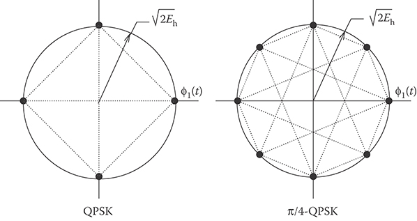
FIGURE 5.5 Complex signal-space diagram QPSK and π/4-DQPSK signals.

The power density spectrum of QPSK and π/4-QPSK is given by

S s ˜ s ˜ (f) = A 2 2 T | H a (f) | 2 . (5.23)

$S_{\tilde{s} \tilde{s}} (f) = \frac{A^{2}}{2 T} {| H_{a} (f) |}^{2} . (5.23)$

Note that π/4-DQPSK has the same power spectrum as QPSK. Of course π/4-DQPSK has a lower PAPR than QPSK.

Images

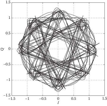
FIGURE 5.6 Phaser diagram for π/4-DQPSK with root raised cosine amplitude pulse shaping; β = 0.5.

5.5 Continuous Phase Modulation, Minimum Shift Keying, and GMSK

Continuous phase modulation (CPM) refers to a broad class of FM techniques where the carrier phase varies in a continuous manner. A comprehensive treatment of CPM is provided in Reference 2. CPM schemes are attractive because they have constant envelope and excellent spectral characteristics. The complex envelope of a CPM waveform has the general form

s ˜ (t) = A e j (ϕ (t) + θ 0), (5.24)

$\tilde{s} (t) = A e^{j (ϕ (t) + θ_{0})}, (5.24)$

where A is the amplitude, θ₀ is initial carrier phase at t = 0, and

ϕ (t) = 2 π h \int 0 t \sum k = 0 \infty x k h f (τ - k T) d τ (5.25)

$ϕ (t) = 2 π h \int_{0}^{t} \sum_{k = 0}^{\infty} x_{k} h_{f} (τ - k T) d τ (5.25)$

is the excess phase, h is the modulation index, {x_k} is the data symbol sequence, h_f(t) is the frequency shaping pulse, and T is the baud period. The CPM waveform can be written in the standard form

s ˜ (t) = A \sum n b (t - n T, x n) (5.26)

$\tilde{s} (t) = A \sum_{n} b (t - n T, x_{n}) (5.26)$

where

b (t, x n) = e j 2 π h \int t 0 \sum \infty k = 0 x k h f (τ - k T) d τ u T (t) (5.27)

$b (t, x_{n}) = e^{j 2 π h \int_{0}^{t} \sum_{k = 0}^{\infty} x_{k} h_{f} (τ - k T) d τ} u_{T} (t) (5.27)$

x_n = (x_n, x_n−1, …, x₀), and we have assumed an initial phase θ₀ = 0. CPM waveforms have the following properties:

The data symbols are chosen from the alphabet {±1, ±3, …, ±(M − 1)}, where M is the modulation alphabet size and M is even.
h is the modulation index and is directly proportional to the peak and/or average frequency deviation from the carrier. The instantaneous frequency deviation from the carrier is

$f dev (t) = 1 2 π d ϕ ( t ) d t = h \sum k = 0 \infty x k h f (t - k T) . (5.28)$ $f_{dev} (t) = \frac{1}{2 π} \frac{d ϕ (t)}{d t} = h \sum_{k = 0}^{\infty} x_{k} h_{f} (t - k T) . (5.28)$
h_f(t) is the frequency shaping function, which is zero for t < 0 and t > LT, and normalized to have an area equal to 1/2. Full response CPM has L = 1, while partial response CPM has L > 1.

5.5.1 Minimum Shift Keying

Minimum shift keying (MSK) is a special form of binary CPM (x_k ∈ {−1, +1}) that uses a rectangular frequency shaping pulse h_f(t) = (1/2T)u_T(t), and a modulation index h = 1/2. In this case,

b (t, x n) = e j (π 2 \sum n - 1 k = 0 x k + π 2 x n t T) u T (t) . (5.29)

$b (t, x_{n}) = e^{j (\frac{π}{2} \sum_{k = 0}^{n - 1} x_{k} + \frac{π}{2} x_{n} \frac{t}{T})} u_{T} (t) . (5.29)$

where u_T(t) = u(t) - u(t - T) and u(t) is the unit step function.

Images

FIGURE 5.7 Phase-trellis for MSK.

The MSK waveform can be described by the phase trellis diagram shown in Figure 5.7 which plots the time behavior of the excess phase

ϕ (t) = π 2 \sum k = 0 n - 1 x k + π 2 x n t - n T T . (5.30)

$ϕ (t) = \frac{π}{2} \sum_{k = 0}^{n - 1} x_{k} + \frac{π}{2} x_{n} \frac{t - n T}{T} . (5.30)$

At the end of each symbol interval the excess phase φ(t) takes on values that are integer multiples of π/2. Since excess phases that differ by integer multiples of 2π are indistinguishable, the values taken by φ(t) at the end of each symbol interval belong to the finite set {0, π/2, π, 3π/2}.

An interesting property of MSK can be observed from the MSK bandpass waveform. The bandpass waveform on the interval [nT,(n + 1)T] can be obtained from Equation 5.29 as

s (t) = A cos (2 π f c t + π 2 \sum k = 0 n - 1 x k + π 2 x n t - n T T) = A cos (2 π (f c + x n 4 T) t + π 2 \sum k = 0 n - 1 x k - π n 2 x n) . (5.31)

$\begin{matrix} s (t) = A \cos (2 π f_{c} t + \frac{π}{2} \sum_{k = 0}^{n - 1} x_{k} + \frac{π}{2} x_{n} \frac{t - n T}{T}) \\ = A \cos (2 π (f_{c} + \frac{x_{n}}{4 T}) t + \frac{π}{2} \sum_{k = 0}^{n - 1} x_{k} - \frac{π n}{2} x_{n}) . \end{matrix} (5.31)$

Observe that the MSK bandpass waveform has one of two possible frequencies in each baud interval

f L = f c - 1 4 T and f U = f c + 1 4 T (5.32)

$f_{L} = f_{c} - \frac{1}{4 T} and f_{U} = f_{c} + \frac{1}{4 T} (5.32)$

depending on the data symbol x_n. The difference between these two frequencies is f_U − f_L = 1/(2T). This is the minimum frequency separation to ensure orthogonality between two cophased sinusoids of duration T and, hence, the name minimum shift keying.

Another interesting representation for MSK waveforms can be obtained by using Laurent's decomposition [3] to express the MSK complex envelope in the quadrature form

s ˜ (t) = A \sum n b (t - 2 n T, x n), (5.33)

$\tilde{s} (t) = A \sum_{n} b (t - 2 n T, x_{n}), (5.33)$

where

b (t, x n) = x ˆ 2 n + 1 h a (t - T) + j x ˆ 2 n h a (t) (5.34)

$b (t, x_{n}) = {\hat{x}}_{2 n + 1} h_{a} (t - T) + j {\hat{x}}_{2 n} h_{a} (t) (5.34)$

and where xn=(xˆ2n+1,xˆ2n) $x_{n} = ({\hat{x}}_{2 n + 1}, {\hat{x}}_{2 n})$ ,

x ˆ 2 n = x ˆ 2 n - 1 x 2 n (5.35)

${\hat{x}}_{2 n} = {\hat{x}}_{2 n - 1} x_{2 n} (5.35)$

x ˆ 2 n + 1 = - x ˆ 2 n x 2 n + 1 (5.36)

${\hat{x}}_{2 n + 1} = - {\hat{x}}_{2 n} x_{2 n + 1} (5.36)$

x ˆ - 1 = 1 (5.37)

${\hat{x}}_{- 1} = 1 (5.37)$

and

h a (t) = sin (π t 2 T) u 2 T (t) . (5.38)

$h_{a} (t) = \sin (\frac{π t}{2 T}) u_{2 T} (t) . (5.38)$

The sequences, {xˆ2n} ${{\hat{x}}_{2 n}}$ and {xˆ2n+1} ${{\hat{x}}_{2 n + 1}}$ , are independent binary symbol sequences taking on values from the set {−1, +1}. The symbols xˆ2n ${\hat{x}}_{2 n}$ and xˆ2n+1 ${\hat{x}}_{2 n + 1}$ are transmitted on the quadrature branches with a half-sinusoid (HS) amplitude shaping pulse of duration 2T s and an offset of Ts. Hence, MSK is equivalent to offset quadrature amplitude shift keying (OQASK) with HS amplitude pulse shaping. This linear representation of MSK is useful in practice for linear detection of MSK waveforms.

To obtain the power density spectrum of MSK, we observe from Equation 5.34 that the MSK baseband signal has the quadrature form

s ˜ (t) = A \sum n b (t - 2 n T, x n), (5.39)

$\tilde{s} (t) = A \sum_{n} b (t - 2 n T, x_{n}), (5.39)$

where

b (t, x n) = x ˆ 2 n + 1 h a (t - T) + j x ˆ 2 n h a (t) (5.40)

$b (t, x_{n}) = {\hat{x}}_{2 n + 1} h_{a} (t - T) + j {\hat{x}}_{2 n} h_{a} (t) (5.40)$

h a (t) = sin (π t 2 T) u 2 T (t), (5.41)

$h_{a} (t) = \sin (\frac{π t}{2 T}) u_{2 T} (t), (5.41)$

xn=(xˆ2n+1,xˆ2n) $x_{n} = ({\hat{x}}_{2 n + 1}, {\hat{x}}_{2 n})$ is a sequence of odd–even pairs assuming values from the set {±1, ±1}, and T is the bit period. The Fourier transform of Equation 5.40 is

B (f, x n) = (x ˆ 2 n + 1 e - j 2 π f T + j x ˆ 2 n) H a (f) . (5.42)

$B (f, x_{n}) = ({\hat{x}}_{2 n + 1} e^{- j 2 π f T} + j {\hat{x}}_{2 n}) H_{a} (f) . (5.42)$

Since the data sequence is zero-mean and uncorrelated, the MSK psd is

S b, 0 (f) = 1 2 E [| B (f, x 0) | 2] = 1 2 E [x ˆ 21 + x ˆ 20] | H a (f) | 2 = | H a (f) | 2 . (5.43)

$\begin{matrix} S_{b, 0} (f) = \frac{1}{2} E [{| B (f, x_{0}) |}^{2}] \\ = \frac{1}{2} E [{\hat{x}}_{1}^{2} + {\hat{x}}_{0}^{2}] {| H_{a} (f) |}^{2} \\ = {| H_{a} (f) |}^{2} . \end{matrix} (5.43)$

The Fourier transform of the HS pulse in Equation 5.38 is

H a (f) = 2 T π ( 1 - ( 4 f ​ T ) 2 ) (1 + e - j 4 π f T) . (5.44)

$H_{a} (f) = \frac{2 T}{π (1 - {(4 f T)}^{2})} (1 + e^{- j 4 π f T}) . (5.44)$

Hence, the power spectrum becomes

S s ˜ s ˜ (f) = A 2 T ∣ ∣ ∣ ∣ ​ H a (f) ​ ∣ ∣ ∣ ∣ 2 = 16 A 2 T π 2 [cos 2 ( 2 π f T ) 1 - ( 4 f T ) 2] 2 ​ . (5.45)

$S_{\tilde{s} \tilde{s}} (f) = \frac{A^{2}}{T} | H_{a} (f) |^{2} = \frac{16 A^{2} T}{π^{2}} {[\frac{\cos^{2} (2 π f T)}{1 - {(4 f T)}^{2}}]}^{2} . (5.45)$

The PSD of MSK is plotted in Figure 5.10. Observe that an MSK signal has fairly large sidelobes compared to π/4-QPSK with a truncated square root raised cosine pulse (cf. Figure 5.4).

5.5.2 Gaussian Minimum Shift Keying

The MSK power spectrum has a relatively broad main lobe and slow roll-off of side lobes. A more compact power spectrum can be achieved by low-pass filtering the MSK modulating signal

x (t) = \sum n = - \infty \infty x n h f (t - n T) = 1 2 T \sum n = - \infty \infty x n u T (t - n T) (5.46)

$x (t) = \sum_{n = - \infty}^{\infty} x_{n} h_{f} (t - n T) = \frac{1}{2 T} \sum_{n = - \infty}^{\infty} x_{n} u_{T} (t - n T) (5.46)$

prior to FM as shown in Figure 5.8. Such filtering suppresses the higher-frequency components in x(t) thus yielding a more compact power spectrum. GMSK is a special type of partial response CPM that uses a low-pass premodulation filter having the transfer function [4]

H (f) = exp {- (f B) 2 ln 2 2}, (5.47)

$H (f) = \exp {- {(\frac{f}{B})}^{2} \frac{\ln 2}{2}}, (5.47)$

where B is the 3 dB bandwidth of the filter. It is apparent that H( f ) is shaped like a Gaussian probability density function with mean f = 0 and, hence, the name “Gaussian” MSK. Convolving the rectangular pulse

1 2 T rect (t / T) = 1 2 T u T (t + T / 2)

$\frac{1}{2 T} rect (t / T) = \frac{1}{2 T} u_{T} (t + T / 2)$

with the corresponding filter impulse response h(t) yields the frequency shaping pulse

h f (t) = 1 2 T 2 π ln 2 - - - \sqrt (B T) \int t / T - 1 / 2 t / T + 1 / 2 exp {- 2 π 2 ( B T ) 2 x 2 ln 2} d x = 1 2 T [Q (t / T - 1 / 2 σ) - Q (t / T + 1 / 2 σ)], (5.48)

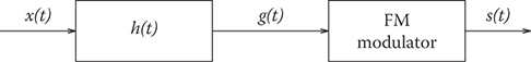
$\begin{matrix} h_{f} (t) = \frac{1}{2 T} \sqrt{\frac{2 π}{\ln 2}} (B T) \int_{t / T - 1 / 2}^{t / T + 1 / 2} \exp {- \frac{2 π^{2} {(B T)}^{2} x^{2}}{\ln 2}} d x \\ = \frac{1}{2 T} [Q (\frac{t / T - 1 / 2}{σ}) - Q (\frac{t / T + 1 / 2}{σ})], \end{matrix} (5.48)$

Images

FIGURE 5.8 Premodulation filtered MSK. The MSK modulating signal is low-pass filtered to remove the high-frequency components prior to FM.

Images

FIGURE 5.9 GMSK frequency shaping pulse for various normalized premodulation filter bandwidths BT.

where

Q (α) = \int \infty α 1 2 π - - \sqrt e - x 2 d x (5.49)

$Q (α) = \int_{α}^{\infty} \frac{1}{\sqrt{2 π}} e^{- x^{2}} d x (5.49)$

σ 2 = ln 2 4 π 2 ( B T ) 2 . (5.50)

$σ^{2} = \frac{\ln 2}{4 π^{2} {(B T)}^{2}} . (5.50)$

Figure 5.9 plots the GMSK frequency shaping pulse (truncated to 5T and time shifted by 2.5T to yield a causal pulse) for various normalized premodulation filter bandwidths BT. The popular GSM cellular standard uses GMSK with BT = 0.3.

The power density spectrum of GMSK is quite difficult to obtain, but can be computed by using published methods [5]. Figure 5.10 plots the power density spectrum for BT = 0.2, 0.25, and 0.3, obtained from K. Wesolowski (private comm., 1994). Observe that the spectral sidelobes are greatly reduced by the Gaussian low-pass filter.

5.6 Orthogonal Frequency Division Multiplexing

Orthogonal frequency division multiplexing (OFDM) is a block modulation scheme where data symbols are transmitted in parallel on orthogonal subcarriers. A block of N data symbols, each of duration T_s, is converted into a block of N parallel data symbols, each of duration T = NT_s. The N parallel data symbols modulate N subcarriers that are spaced in frequency 1/T Hz apart. The OFDM complex envelope is given by

s ˜ (t) = A \sum n b (t - n T, x n), (5.51)

$\tilde{s} (t) = A \sum_{n} b (t - n T, x_{n}), (5.51)$

where

b (t, x n) = u T (t) \sum k = 0 N - 1 x n k e j 2 π k t T (5.52)

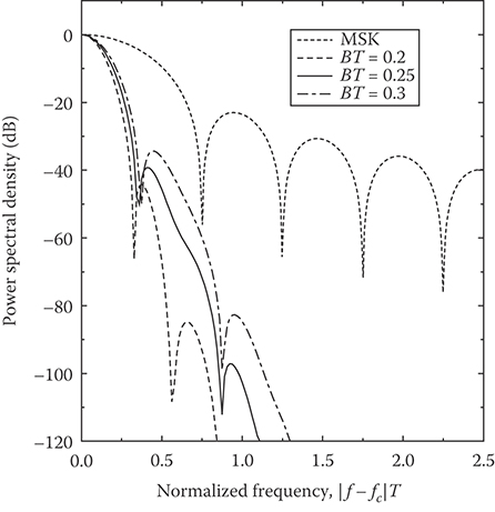
$b (t, x_{n}) = u_{T} (t) \sum_{k = 0}^{N - 1} x_{n_{k}} e^{j \frac{2 π k t}{T}} (5.52)$

Images

FIGURE 5.10 Power density spectrum of MSK and GMSK.

n is the block index, k is the subcarrier index, N is the number of subcarriers, and xn={xn0,xn1,…,xnN−1} $x_{n} = {x_{n_{0}}, x_{n_{1}}, \dots, x_{n_{N - 1}}}$ is the data symbol block at epoch n. The data symbols xnk $x_{n_{k}}$ are usually chosen from a QAM or PSK signal constellation, although any 2-D signal constellation can be used. The 1/T Hz frequency separation of the subcarriers ensures that the corresponding subchannels are mutually orthogonal regardless of the random phases that are imparted by the data modulation.

A cyclic extension (or guard interval) is usually added to the OFDM waveform in Equations 5.51 and 5.52 to combat delay spread. The cyclic extension can be in the form of either a cyclic prefix or a cyclic suffix. With a cyclic suffix, the OFDM complex envelope becomes

s ˜ g (t) = {s ˜ (t), s ˜ (t - T), 0 \leq t \leq T T \leq t \leq (1 + α g) T, (5.53)

${\tilde{s}}_{g} (t) = {\begin{array}{l} \tilde{s} (t), & 0 \leq t \leq T \\ \tilde{s} (t - T), & T \leq t \leq (1 + α_{g}) T, \end{array} (5.53)$

where α_gT is the length of the guard interval and s˜(t) $\tilde{s} (t)$ is defined in Equations 5.51 and 5.52. The OFDM waveform with cyclic suffix can be rewritten in the standard form

s ˜ g (t) = A \sum n b (t - n T g, x n), (5.54)

${\tilde{s}}_{g} (t) = A \sum_{n} b (t - n T_{g}, x_{n}), (5.54)$

where

b (t, x n) = u T (t) \sum k = 0 N - 1 x n k e j 2 π k t T + u α g T (t - T) \sum k = 0 N - 1 x n k e j 2 π k ( t - T ) T, (5.55)

$b (t, x_{n}) = u_{T} (t) \sum_{k = 0}^{N - 1} x_{n_{k}} e^{j \frac{2 π k t}{T}} + u_{α_{g} T} (t - T) \sum_{k = 0}^{N - 1} x_{n_{k}} e^{j \frac{2 π k (t - T)}{T}}, (5.55)$

and T_g = (1 + α_g)T is the OFDM symbol period with the addition of the guard interval. Likewise, with a cyclic prefix, the OFDM complex envelope becomes

s ˜ g (t) = {s ˜ (t + T), s ˜ (t), - α g T \leq t \leq 0 0 \leq t \leq T, (5.56)

${\tilde{s}}_{g} (t) = {\begin{array}{l} \tilde{s} (t + T), & - α_{g} T \leq t \leq 0 \\ \tilde{s} (t), & 0 \leq t \leq T \end{array}, (5.56)$

and

b (t, x n) = u α g T (t + α g T) \sum k = 0 N - 1 x n k e j 2 π k ( t + T ) T + u T (t) \sum k = 0 N - 1 x n k e j 2 π k t T . (5.57)

$b (t, x_{n}) = u_{α_{g} T} (t + α_{g} T) \sum_{k = 0}^{N - 1} x_{n_{k}} e^{j \frac{2 π k (t + T)}{T}} + u_{T} (t) \sum_{k = 0}^{N - 1} x_{n_{k}} e^{j \frac{2 π k t}{T}} . (5.57)$

5.6.1 FFT Implementation of OFDM

A key advantage of using OFDM is that the baseband modulator can be implemented by using an inverse discrete-time Fourier transform (IDFT). In practice, an inverse fast Fourier transform (IFFT) algorithm is used to implement the IDFT. Consider the OFDM complex defined by Equations 5.51 and 5.52. During the interval nT ≤ t ≤ (n + 1)T, the complex envelope has the form

s ˜ (t) = A u T (t - n T) \sum k = 0 N - 1 x n k e j 2 π k ( t - n T ) T = A u T (t - n T) \sum k = 0 N - 1 x n k e j 2 π k t N T s, n T \leq t \leq (n + 1) T . (5.58)

$\begin{matrix} \tilde{s} (t) = A u_{T} (t - n T) \sum_{k = 0}^{N - 1} x_{n_{k}} e^{\frac{j 2 π k (t - n T)}{T}} \\ = A u_{T} (t - n T) \sum_{k = 0}^{N - 1} x_{n_{k}} e^{\frac{j 2 π k t}{N T_{s}}}, n T \leq t \leq (n + 1) T . \end{matrix} (5.58)$

Now suppose that the complex envelope in Equation 5.58 is sampled at synchronized T_s second intervals to yield the sample sequence

X n m = s ˜ (m T s) = A \sum k = 0 N - 1 x n k e j 2 π k m N, m = 0, 1, \dots, N - 1. (5.59)

$X_{n_{m}} = \tilde{s} (m T_{s}) = A \sum_{k = 0}^{N - 1} x_{n_{k}} e^{\frac{j 2 π k m}{N}}, m = 0, 1, \dots, N - 1. (5.59)$

Observe that the vector Xn={Xnm}N−1m=0 $X_{n} = {X_{n_{m}}}_{m = 0}^{N - 1}$ is the IDFT of the vector Axn=A{xnk}N−1k=0 $A x_{n} = A {x_{n_{k}} }_{k = 0}^{N - 1}$ . In contrast to conventional notation, the lower-case vector Ax_n is used to represent the coefficients in the frequency domain, while the upper-case vector X_n is used to represent the coefficients in the time domain.

As mentioned earlier, a cyclic extension (or guard interval) is usually added to the OFDM waveform as described in Equations 5.54 and 5.55 to combat delay spread. When a cyclic suffix is used, the corresponding sample sequence is

X g n m = X n (m) N (5.60)

$X_{n_{m}}^{g} = X_{n_{{(m)}_{N}}} (5.60)$

= A \sum k = 0 N - 1 x n k e j 2 π k m N, m = 0, 1, \dots, N + G - 1, (5.61)

$= A \sum_{k = 0}^{N - 1} x_{n_{k}} e^{\frac{j 2 π k m}{N}}, m = 0, 1, \dots, N + G - 1, (5.61)$

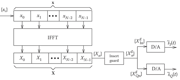
where G is the length of the guard interval in samples, and (m)_N is the residue of m modulo N. This gives the vector Xgn={Xgnm}N+G−1m=0 $X_{n}^{g} = {X_{n_{m}}^{g}}_{m = 0}^{N + G - 1}$ , where the values in the first and last G coordinates of the vector Xgn $X_{n}^{g}$ are the same. Likewise, when a cyclic prefix is used, the corresponding sample sequence is

Images

FIGURE 5.11 Block diagram of IDFT-based baseband OFDM modulator with guard interval insertion and digital-to-analog conversion.

X g n m = X n (m) N (5.62)

$X_{n_{m}}^{g} = X_{n_{{(m)}_{N}}} (5.62)$

= A \sum k = 0 N - 1 x n k e j 2 π k m N, m = - G, \dots, - 1, 0, 1, \dots, N - 1. (5.63)

$= A \sum_{k = 0}^{N - 1} x_{n_{k}} e^{\frac{j 2 π k m}{N}}, m = - G, \dots, - 1, 0, 1, \dots, N - 1. (5.63)$

This yields the vector Xgn={Xgnm}N−1m=−G $X_{n}^{g} = {X_{n_{m}}^{g}}_{m = - G}^{N - 1}$ , where again the first and last G coordinates of the vector Xgn $X_{n}^{g}$ are the same. The sample duration after insertion of the guard interval, Tgs $T_{s}^{g}$ , is compressed in time such that (N+G)Tgs=NTs $(N + G) T_{s}^{g} = N T_{s}$ .

The OFDM complex envelope can be generated by splitting the complex-valued output vector X_m into its real and imaginary parts, ℜ(X_n) and I(Xn) $ℑ (X_{n})$ , respectively. The sequences {R(Xnm)} ${ℜ (X_{n_{m}})}$ and {I(Xnm)} ${ℑ (X_{n_{m}})}$ are then input to a pair of balanced digital-to-analog converters (DACs) to generate the real and imaginary components s˜I(t) ${\tilde{s}}_{I} (t)$ and s˜Q(t) ${\tilde{s}}_{Q} (t)$ , respectively, of the complex envelope s˜(t) $\tilde{s} (t)$ , during the time interval nT ≤ t ≤ (n + 1)T. As shown in Figure 5.11, the OFDM baseband modulator consists of an IFFT operation, followed by guard interval insertion and digital-to-analog conversion.

It is instructive to realize that the waveform generated by using the IDFT OFDM baseband modulator is not exactly the same as the waveform generated from the analog waveform definition of OFDM. Consider for example, the OFDM waveform without a cyclic guard in Equations 5.51 and 5.52. The analog waveform definition uses the rectangular amplitude shaping pulse u_T(t) that is strictly time limited to T seconds. Hence, the corresponding power spectrum will have infinite bandwidth, and any finite sampling rate of the complex envelope will necessarily lead to aliasing and imperfect reconstruction.

5.6.2 Power Spectrum of OFDM

To compute the power spectrum of OFDM, recall that the OFDM waveform with guard interval is given by Equations 5.54 and 5.55. The data symbols xnk $x_{n_{k}}$ , k = 0, … ,N − 1 that modulate the N subcarriers are assumed to have zero mean, variance σ2x=1/2 E[|xk,n|2] $σ_{x}^{2} = 1 / 2 E [| x_{k, n} |^{2}]$ , and they are mutually uncorrelated. In this case, the psd of the OFDM waveform is

S s ˜ s ˜ (f) = A 2 T g S b, 0 (f), (5.64)

$S_{\tilde{s} \tilde{s}} (f) = \frac{A^{2}}{T_{g}} S_{b, 0} (f), (5.64)$

where

S b, 0 (f) = 1 2 E [| B (f, x 0) | 2], (5.65)

$S_{b, 0} (f) = \frac{1}{2} E [{| B (f, x_{0}) |}^{2}], (5.65)$

and

B (f, x 0) = \sum k = 0 N - 1 x 0 k T sinc (f T - k) + \sum k = 0 N - 1 x 0 k α g T sinc (α g (f T - k)) e j 2 π f T . (5.66)

$B (f, x_{0}) = \sum_{k = 0}^{N - 1} x_{0_{k}} T sinc (f T - k) + \sum_{k = 0}^{N - 1} x_{0_{k}} α_{g} T sinc (α_{g} (f T - k)) e^{j 2 π f T} . (5.66)$

Substituting Equation 5.66 into Equation 5.65 along with T = NT_s yields the result

S s ˜ s ˜ (f) = σ 2 x A 2 T (1 1 + α g \sum k = 0 N - 1 sinc 2 (N f T s - k) + α 2 g 1 + α g \sum k = 0 N - 1 sinc 2 (α g (N f T s - k)) + 2 α g 1 + α g cos (2 π N f T s) \sum k = 0 N - 1 sinc (N f T s - k) sinc (α g (N f T s - k))) . (5.67)

$\begin{matrix} S_{\tilde{s} \tilde{s}} (f) = σ_{x}^{2} A^{2} T (\frac{1}{1 + α_{g}} \sum_{k = 0}^{N - 1} {sinc}^{2} (N f T_{s} - k) + \frac{α_{g}^{2}}{1 + α_{g}} \sum_{k = 0}^{N - 1} {sinc}^{2} (α_{g} (N f T_{s} - k)) \\ + \frac{2 α_{g}}{1 + α_{g}} \cos (2 π N f T_{s}) \sum_{k = 0}^{N - 1} sinc (N f T_{s} - k) sinc (α_{g} (N f T_{s} - k))) . \end{matrix} (5.67)$

The OFDM PSD is plotted in Figure 5.12 for N = 16, α_g = 0.25.

It is interesting to examine the OFDM power spectrum, when the OFDM complex envelope is generated by using an IDFT baseband modulator followed by a balanced pair DACs as shown in Figure 5.11. The output of the IDFT baseband modulator is given by {Xg}={Xgm,n} ${X^{g}} = {X_{m, n}^{g}}$ , where m is the block index and

X g m, n = X m, (n) N (5.68)

$X_{m, n}^{g} = X_{m, {(n)}_{N}} (5.68)$

= A \sum k = 0 N - 1 x m, k e j 2 π k n N, n = 0, 1, \dots, N + G - 1. (5.69)

$= A \sum_{k = 0}^{N - 1} x_{m, k} e^{\frac{j 2 π k n}{N}}, n = 0, 1, \dots, N + G - 1. (5.69)$

Images

FIGURE 5.12 PSD of OFDM with N = 16, α_g = 0.25.

The power spectrum of the sequence {X^g} can be calculated by first determining the discrete-time autocorrelation function of the time-domain sequence {X^g} and then taking a discrete-time Fourier transform of the discrete-time autocorrelation function. The PSD of the OFDM complex envelope with ideal DACs can be obtained by applying the resulting power spectrum to an ideal low-pass filter with a cutoff frequency of 1/(2Tgs) Hz $1 / (2 T_{s}^{g}) Hz$ .

The discrete-time autocorrelation function of the sequence {X^g} is

ϕ X g X g (ℓ) = ⎧ ⎩ ⎨ ⎪ ⎪ ⎪ ⎪ A σ 2 X G N + G A σ 2 X 0 ℓ = 0 ℓ = - N, N otherwise . (5.70)

$ϕ_{X^{g} X^{g}} (ℓ) = {\begin{array}{l} A σ_{X}^{2} & ℓ = 0 \\ \frac{G}{N + G} A σ_{X}^{2} & ℓ = - N, N \\ 0 & otherwise \end{array} . (5.70)$

Taking the discrete-time Fourier transform of the discrete-time autocorrelation function in Equation 5.70 gives

S X g X g (f) = A σ 2 x (1 + G N + G e - j 2 π f N T g s + G N + G e j 2 π f N T g s) = A σ 2 x (1 + 2 G N + G cos (2 π f N T g s)) . (5.71)

$\begin{matrix} S_{X^{g} X^{g}} (f) = A σ_{x}^{2} (1 + \frac{G}{N + G} e^{- j 2 π f N T_{s}^{g}} + \frac{G}{N + G} e^{j 2 π f N T_{s}^{g}}) \\ = A σ_{x}^{2} (1 + \frac{2 G}{N + G} \cos (2 π f N T_{s}^{g})) . \end{matrix} (5.71)$

Finally, we assume that the sequence ${X^{g}} = {X_{m, n}^{g}}$ is passed through a pair of ideal DACs. The ideal DAC is a low-pass filter with cutoff frequency $1 / (2 T_{s}^{g})$ . Therefore, the OFDM complex envelope has the PSD

$S_{\tilde{s} \tilde{s}} (f) = A σ_{x}^{2} (1 + \frac{2 G}{N + G} \cos (2 π f N T_{s}^{g})) rect (f T_{s}^{g}) . (5.72)$

Figure 5.13 plots the PSD for N = 16 and G = 4.

Images

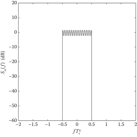
FIGURE 5.13 PSD of IDFT-based OFDM with N = 16, G = 4.

Finally, we note that the PSD plotted in Figure 5.13 assumes an ideal DAC. A practical DAC with a finite-length reconstruction filter will introduce sidelobes into the spectrum. We note that sidelobes are an inherent feature of the continuous-time OFDM waveform in Equations 5.54 and 5.55 due to the use of rectangular amplitude pulse shaping on the subcarriers. However, sidelobes are introduced into the waveform generated with the IDFT implementation by the nonideal (practical) DAC.

5.7 Summary and Conclusions

A variety of modulation schemes are employed in digital communication systems. Wireless modulation schemes in particular must have a compact power density spectrum, while at the same time providing a good bit error rate performance in the presence of channel impairments such as cochannel interference and fading. This chapter has presented a variety of modulation schemes along with their power spectra.

References

1. G. L. Stüber, Principles of Mobile Communication, 3rd edn, Springer Science + Business Media, 2011.

2. J. B. Anderson, T. Aulin, and C. E. Sundberg, Digital Phase Modulation. New York, NY: Plenum, 1986.

3. P. A. Laurent, Exact and approximate construction of digital phase modulations by superposition of amplitude modulated pulses (AMP). IEEE Trans. Commun., 34, 150–160, 1986.

4. K. Murota and K. Hirade, GMSK modulation for digital mobile radio telephony. IEEE Trans. Commun., 29(July), 1044–1050, 1981.

5. G. J. Garrison, A power spectral density analysis for digital FM. IEEE Trans. Commun., 23(November), 1228–1243, 1975.

Table of Contents for
5 Modulation Methods

5

Modulation Methods

5.1 Introduction

5.2 Basic Description of Modulated Signals

5.3 Quadrature Amplitude Modulation

5.3.1 QAM Signal Constellations

5.3.2 Root Raised Cosine Pulse Shaping

5.3.3 Power Spectrum of QAM

5.4 Phase Shift Keying and π/4-QDPSK

5.5 Continuous Phase Modulation, Minimum Shift Keying, and GMSK

5.5.1 Minimum Shift Keying

5.5.2 Gaussian Minimum Shift Keying

5.6 Orthogonal Frequency Division Multiplexing

5.6.1 FFT Implementation of OFDM

5.6.2 Power Spectrum of OFDM

5.7 Summary and Conclusions

References

Further Reading

Table of Contents for 5 Modulation Methods

Create new playlist

Sign In

Sign Up

5

Table of Contents for
5 Modulation Methods