
13
Introduction to Spread Spectrum Systems
Dinesh Rajan
13.2 Direct Sequence Spread Spectrum
13.3 Frequency Hopping Spread Spectrum
13.4 Applications of Spread Spectrum
DS–CDMA-Based Cellular Systems
Synchronization Issues in Spread Spectrum Systems
13.1 Introduction
Spread spectrum signals typically refer to signals that use a bandwidth that is significantly higher than the minimum bandwidth required to transmit that information sequence. Although bandwidth is a precious commodity, increasing the bandwidth of the signal prior to transmission results in several advantages: (i) The resulting power spectral density (PSD) of the spread signal is lower than the PSD of the signal prior to spreading. (ii) The resulting signal is more resistant to narrow band interference/jamming. (iii) The signal has a low probability of being intercepted. (iv) The spread signal is readily suitable for multiple access. These advantages have resulted in several military and commercial applications for spread spectrum systems.
The early developments in spread spectrum systems were primarily in military applications, where the low probability of intercept and antijam features were especially useful. Subsequently, they found utility in the commercial area. For instance, commercial applications of spread spectrum in the cellular wide area networks are similar to the military predecessors in many aspects. However, a few specific innovations enable them to attain superior performance. For instance, in the cellular application, primary innovations include the use of universal frequency reuse with intelligent adaptive power control and the use of noise-like signal waveforms. Further, wireless personal area networks such as Zigbee [1,2] and Bluetooth networks [3,4] are based on spread spectrum technology.
Consider a simple multiuser spread spectrum system where the received signal is at power P and the interference from (M – 1) users equals (M – 1)P. Given a system bandwidth of W Hz, the received Eb/N0 can be calculated as (P/R)/(N + (M – 1)P/W), where R is the data rate in bits per second and N is the noise power spectral density. Thus, the desired minimum value of Eb/N0 can be satisfied in the presence of large number of users, if the bandwidth W is appropriately scaled. A similar analysis can be used to demonstrate the advantages of spread spectrum system, if the interference is from an intentional narrow band jammer.
This chapter is organized as follows. In Section 13.2, we discuss direct sequence spread spectrum systems. In Section 13.3, we focus on frequency hopping systems. Applications of spread spectrum are discussed in Section 13.4 followed by some brief concluding remarks in Section 13.5.
13.2 Direct Sequence Spread Spectrum
In a direct sequence (DS) code division multiple access (CDMA) system, the data sequence is multiplied by a pseudo-random signal before transmission. This pseudo-random signal is derived from a spreading code or spreading sequence. Each bit of the spreading sequence is also sometimes referred to as a chip. The time period, Tc, of a chip is usually much smaller than the symbol time period, Ts and the ratio L = Ts/Tc is referred to as the bandwidth expansion factor. In many systems this value L is selected to be an integer. The value L also represents the maximum number of orthogonal users that can be supported without any multiuser interference.
In a multiuser uplink scenario, the signals transmitted by the various users are not synchronous with each other. However, for simplicity of exposition, we first consider a synchronous DS–CDMA system. In a synchronous system, the signals of all the users are perfectly synchronized at the receiver. Such a model is appropriate for a downlink cellular system in which the signals of all the users are transmitted from a single base station. Let there be K users and let the bit sequence of the kth user be denoted by bk(n). Let ck(t) denote the spreading signal used to modulate the kth user's signal. Let the channel from the kth user to the central receiver be denoted by Ak. The received signal, r(t), is given by
where z(t) represents the additive noise at the receiver and is typically modeled as a Gaussian process. The spreading sequence, ck(t) is usually nonzero only in the interval 0 ≤ t < Ts. Thus, there is no inter-symbol interference (ISI) in the system. This code sequence is generated based on the PN spreading sequence and a pulse shaping signal p(t) which is nonzero in the interval 0 ≤ t < Tc. An example of the time-domain and frequency domain representation of the DS-CDMA signal is shown in Figure 13.1a and b, respectively.
Depending on the length of the spreading codes, the sequences are also referred to as long codes or short codes. In a short code DS–CDMA system, the same spreading code is used for all symbols of a particular user. In other words, the spreading code length Lc equals L the bandwidth expansion factor. In this case, the spreading signal ck(t) is given by
In a long code DS–CDMA system, the length of the code Lc is much greater than L the bandwidth expansion factor. In this case, the received signal r(t) is given by
where modulo L and the concatenation of the Lc/L segments of the spreading signal is based on the long spreading code. Many practical systems such as IS-95 and CDMA-2000 use a combination of both a short code and long code. Short orthogonal codes are used to separate the signals of the various users in a cell. Long codes are used for synchronization purposes and to differentiate the signals of users in different cells.
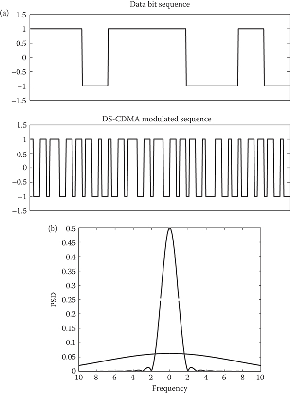
FIGURE 13.1 (a) The time domain representation of a narrow band signal and the equivalent DS-CDMA signal. (b) The frequency domain representation of the same narrow band signal and DS-CDMA signal.
At the receiver, the signal is first typically passed through a set of matched filters (MFs) corresponding to each of the users. The output of the MF corresponding to the nth bit for the kth user is given by
where represents the cross-correlation between the spreading waveforms of user j and user k.
The outputs yk(n) from the MFs essentially represent a discrete time equivalent signal for the DS–CDMA signal. The collection of these outputs is succinctly represented in matrix form as follows:
where R and A represent, respectively, the code correlation and channel gain of the various users. The vector b = [b1 b2 … bK]T represents the information from all users.
In the special case of the cross-correlation between the various spreading waveforms being 0, the multiuser interference in Equation 13.6 is completely eliminated and the channel effectively behaves like K orthogonal single user channels. In general, for nonorthogonal spreading waveforms, the performance of the MF receiver is dependent on the amount of cross correlation and the relative amplitudes of the various users. For instance, the bit error rate (BER) Pe,MF(k) of user k using a MF in the synchronous case is bounded as
If the spreading waveforms of the users are not orthogonal, then a multiuser detector is used to improve the performance [5] over that of a simple MF receiver. The optimum receiver that minimizes the probability of error is the maximum likelihood sequence detector. However, the complexity of such a receiver is high since it involves enumeration of a large set of possible sequences. Two alternate receivers with lower complexity are the linear minimum mean squared error (LMMSE) and the decorrelating receiver. In a decorrelating receiver, the signal in Equation 13.6 is multiplied by the inverse R−1 of the cross-correlation matrix R. The advantage of such a decorrelating receiver is that it completely eliminates the multiuser interference. However, the decorrelating receiver can result in an increase in the effective noise variance. The LMMSE receiver on the other hand offers an optimal trade-off between reducing the multiuser interference and the effective noise. In the LMMSE receiver, the signal in Equation 13.6 is multiplied by M = (R + σ2A−2)−1 and the resulting output is passed through a sign detector (in the case of antipodal signaling). The exact probability of error of the LMMSE receiver has been calculated in Reference 5, but as in the earlier case, its evaluation requires a computational complexity that is exponential in the number of users. Consequently, low complexity approximations for the error rate have been obtained using a Gaussian approximation for the multiuser interference. One such approximation for the error rate for user k is given by
where .
A plot of the BER of the various multiuser detectors is given in Figure 13.2a as a function of the SNR. In this case, each user is assigned a random binary code. It is clear from the figure that the performance of the MF is poor due to the presence of significant multiuser interference. As expected the LMMSE detector performs slightly better than the decorrelating receiver. The variation of the BER with the number of users is given in Figure 13.2b for the various multiuser detectors. Owing to the random nature of the spreading codes used to generate this figure, it can be clearly seen that the BER increases as the number of users increase. In addition to the various multiuser detectors discussed so far, there are several other linear and nonlinear multiuser detectors such as serial or parallel interference cancellation receivers [5].
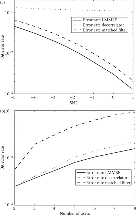
FIGURE 13.2 BER of various multiuser detectors are shown as a function of (a) the SNR and (b) the number of users.
Another advantage of the DS–CDMA systems when used for voice applications is that the voice users are not active for the entire duration of the call. The typical voice activity factor α is lesser than 50% and ensures that the effective interference is only a fraction α of the total interference. Thus, unlike in fixed TDMA systems, the actual interference experienced in a DS–CDMA system is smaller.
The analysis of an asynchronous CDMA system follows along similar lines with some additional modifications. In this case, the received signal is given by
The maximum likelihood sequence detector, LMMSE and decorrelating receivers are defined in a manner similar to the synchronous case. The performance evaluation can also be generalized to this case; however, the analysis is more involved since each bit for a particular user may be affected by portions of 2 bits from each of the other users. In other words, each bit sees interference from 2(K – 1) other bits.
The power spectral density (PSD) of a DS–CDMA system using a raised cosine transmit pulse is shown in Figure 13.1. For reference the PSD of the data sequence as well as a realization of the data sequence and spread sequence are shown in Figure 13.1. The increased bandwidth of DS–CDMA sequence is clearly evident from this figure.
A DS–CDMA signal has good performance even in the presence of a narrow band interference signal. Clearly, the process of spreading at the transmitter ensures that a narrow band signal is now spread over a wider bandwidth. The narrow band interference now additively interferes with the spread CDMA signal. The process of despreading gathers the energy from the spread signal into a narrow band. On the other hand, the despreading operation results in a spreading of the narrow band interference signal over a wider band. Hence, the effective power spectral density of the narrow band interference after despreading is reduced and thus its effect on the CDMA signal is also reduced. If is the energy of the interfering signal, then the effective SNR of the DS–CDMA signal is given by , where N is the length of the spreading code.
It has, however, been shown that the performance of the DS–CDMA signal can be significantly improved by actively suppressing the narrow band interference signal prior to despreading at the receiver [6,7]. These active noise suppression schemes have been widely investigated and can be classified into the following major schemes.
Time domain estimation and interference subtraction. In these methods, an estimator is used to predict the narrow band signal and then subtract this estimated narrow band signal from the spread signal using a notch filter.
Frequency domain filtering. A Fourier transform of the spread signal is first created and then the signal is filtered at a few selected frequencies. The resulting signal is passed through an inverse Fourier transform. The frequencies to filter can be calculated in an adaptive manner, for instance, by selecting spectral components that have energy higher than a certain threshold.
Nonlinear techniques. Unlike the earlier two methods, there are also several nonlinear filtering methods that have been studied in the literature for narrow band interference suppression. One such method uses a decision feedback mechanism to predict the narrow band interference signal and then cancel its effect from the spread signal.
13.3 Frequency Hopping Spread Spectrum
Frequency hopping was first invented during World War II by Hedy Lamarr in a patent titled “Secret Communication System” [8]. In a frequency hopping spread spectrum system, the actual signal transmitted has narrow bandwidth. However, the center frequency of the transmission signal is varied over a wide band. The rate at which the center frequency of the signal is varied determines whether the system is a slow-hopping or fast-hopping system. The variation of the frequency, commonly referred to as hopping pattern, is usually based on a pseudorandom sequence. The advantage of a frequency hopping system is that its performance is not significantly affected by a narrow band interference source, since only the packets that are transmitted when the systems hops at the frequencies of the interfering signal are affected. The FH system also enables multiple point-to-point links in a given location if the hopping sequences used by the various links are effectively different. Note that the difference in the effective hopping pattern used by the various nodes could result from the use of different phases of the same hopping sequence for the various links. A block diagram of a typical FH spread spectrum signal is shown in Figure 13.3.

FIGURE 13.3 Block diagram of a frequency hopping system.
The modulation in an FH system is typically selected to be a form of Frequency Shift Keying (FSK) or Phase Shift Keying (PSK). For instance, in a binary FSK–FH system a binary “0” could be represented by a negative frequency deviation fd from the carrier frequency fc and a binary “1” could be represented by a positive frequency deviation fd from fc. The center frequency fc is varied based on the PN sequence generated. In a MFSK system the frequency spacing between carriers is carefully selected to ensure optimum performance for a given receiver structure. In a noncoherent energy-based detector for the MFSK signal, it is desirable for the various tones representing the bits to be orthogonal to each other. This orthogonality can be achieved by spacing the carriers at integer multiples of 1/Ts. A common arrangement for a FH–MFSK system is to consider nonoverlapping blocks of spectrum of width M · 1/Ts. Each block of this spectrum is assigned to one hopping pattern of the PN code. Such an arrangement of tones is depicted in Figure 13.4. In Figure 13.4, there are N groups of M tones and each of these groups can be selected based on a PN code of length log(N).
As another example, consider a FH–PSK system. Using differential PSK in a FH system, the transmitted bandpass signal s(t) can be represented as
where m(t) is the low-pass signal. This differential PSK signal m(t) can be generated using a pulse shape p(t) as

FIGURE 13.4 One possible arrangement of tones in a M-FSK frequency hopping system.

FIGURE 13.5 Depiction of slow and fast frequency hopping systems.
where is the differential PSK signal. For an 8-ary signal, φk ∈ {0, π/4, π/2, 3π/4, π, 5π/4, 3π/2, 7π/8}. The pulse shape p(t) that is commonly used is the raised cosine pulse [9].
At the receiver, acquisition and tracking of the PN sequence used for frequency hopping is critical for successful decoding of the signal, as discussed in Section 13.4.4. Once the carrier frequency is obtained, the received signal is then converted into baseband in a process that is sometimes called frequency dehopping. The differential PSK signal can then be detected using a noncoherent detector.
In a slow frequency hop system multiple symbols are transmitted on each hop. In contrast, in a fast frequency hop system there are one or more hops for each symbol. A graphical representation of the slow and fast hopping FH systems is shown in Figure 13.5.
The BER of a slow FH system with orthogonal FSK can be derived as
This expression for the BER is derived for the signal transmission in the presence of AWGN. In a fast FH system with M hops per bit, the signal from each of the M subintervals corresponding to a bit are combined together before detection. In this scenario, it turns out that the probability of error is greater than Equation 13.12 and the difference is known as the noncoherent combining loss [9]. The performance of FH systems in fading channels is studied in Reference 10 and the performance in the presence of an interference signal is discussed in Reference 11.
13.3.1 Time Hopping Spread Spectrum
A time hopping spread spectrum (THSS) system is analogous to a frequency hopping spread spectrum system. In a THSS each time slot of duration T is divided into smaller subintervals of length Tm. The coded information bits of the user are transmitted in a pseudo-randomly selected subintervals. Let the information data be at rate R bits/s and the coded rate equals R/r, where r is the rate of the channel code used. Since this rate needs to be transmitted in an interval of length Tm<T, the bandwidth required is increased.
13.4 Applications of Spread Spectrum
In this section, we highlight some of the important applications of spread spectrum signals. We first discuss cellular applications in Section 13.4.1, followed by applications in Bluetooth (Section 13.4.2) and ultrawideband systems (Section 13.4.3). Finally, we discuss synchronization issues in Section 13.4.4.
13.4.1 DS–CDMA-Based Cellular Systems
One of the original applications of DS–CDMA in digital cellular systems is the IS-95 standard. The second-generation cellular technology uses a combination of a Walsh code and a long PN code to spread the data bits. The receiver uses a rake receiver to combine the signal from the various multipaths and boost signal performance. The standard also supports a soft handover process between multiple cells. Subsequently, this standard has been replaced by the CDMA2000 and W-CDMA standards.
13.4.2 Bluetooth
The Bluetooth technology is an excellent example that demonstrates the commercial success of spread spectrum technology in enabling multiple independent peer-to-peer networks to simultaneously operate in the same geographical area. The first version of the Bluetooth standard was released in 1999. It has subsequently been revised multiple times with the latest version being Version 4. Bluetooth is designed as a short range, low energy, and inexpensive means for transferring voice, video and data between two or more devices without any infrastructure support. Bluetooth-based products have appeared in several applications such as hands free calling in cars and mobile phones, wireless game controllers, and wireless computer peripheral devices.
The basic Bluetooth network architecture is a piconet in which upto 8 devices communicate with each other by selecting one of the participating nodes as a master. The remaining nodes in the piconet are labeled as the slave nodes. Bluetooth operates in the 2.4 GHz ISM band and uses 79 channels of 1 MHz bandwidth from 2.402 to 2.48 GHz. Bluetooth is essentially an FH system in which the hopping frequency is determined by the Master node in a piconet from among these 79 frequencies. In addition, Bluetooth also uses an adaptive frequency hopping mechanism [12] to avoid interference from other devices operating in the same frequency band and also to better exploit the frequency-dependent behavior of the wideband channel.
13.4.3 Ultrawideband Systems
Ultrawideband communication systems have a long history with the original transmit signal pulses of very short duration, resulting in very large bandwidths. Subsequently, the need for multiplexing and coexistence of various signals in a given area resulted in the use of narrow band signals of larger time duration. More recent interest in UWB signals is a result of the FCC's decision (followed by similar rules in several other countries) to open up the spectrum from 3.1 to 10.6 GHz for the operation of unlicensed UWB devices.
Ultrawideband systems are loosely defined as systems that transmit information over a bandwidth in excess of the minimum of 500 MHz or using a fractional bandwidth of at least 0.2, that is, the bandwidth exceeds 20% of the center frequency of transmission [13]. These systems include both UWB based radar/imaging systems and short range, high data rate communication systems.
Buoyed by the commercial success of Bluetooth, several companies decided to create a high-speed, ultrawideband personal area communication system to replace wires between the computer and peripherals such as monitors and also between media players and high-definition TVs. The wireless community developed two competing approaches to achieve this goal. The first approach, labeled the multiband OFDM ultrawideband system, uses a combination of OFDM and frequency hopping [14]. The second approach is based on DS–CDMA signaling [15].
While both approaches have their advantages and disadvantages, the lack of a consensus solution was detrimental to the standardization process and to the development of an ecosystem to support this technology and led to the eventual commercial failure. It is the hope of this author that newer ultrawideband systems based on spread spectrum signaling would become available in the near future.
13.4.4 Synchronization Issues in Spread Spectrum Systems
One of the major challenges in a spread spectrum system is to ensure that the PN sequences at the transmitter and receiver are perfectly synchronized. There are several factors that cause an uncertainty in time and frequency between the PN sequences at the transmitter and receiver. For instance, the propagation delay, the use of different clocks and different phases of the carrier cause a temporal shift. Similarly, the Doppler effect due to the relative motion between the transmitter and receiver cause a frequency error.
A maximum-likelihood estimator of the various user's amplitude, phase and delay is given in Reference 16. In most practical system, the PN synchronization is accomplished as a two-step process. In the first step, called as the acquisition step, a coarse alignment of the sequences is obtained. In the second phase, called the tracking phase, fine synchronization is obtained and continually updated. The acquisition is essentially carried out by correlating the received signal with various shifted versions of a copy of the transmitted signal. The goal is to select the shift that results in the maximum value of this correlation. In practice, the value of the correlation becoming higher than a threshold is used to indicate a potential acquisition of the PN signal. The fine synchronization is obtained using for instance a delay locked loop. In this case, the symmetric property of the autocorrelation is used to establish fine synchronization. The received signal is correlated with two versions of the coarse estimated PN sequence with shifts +τ and –τ, respectively. The difference in value of the correlation for these two shifts is used in a feedback loop to obtain and maintain fine synchronization.
13.5 Conclusions
This chapter provides a basic introduction to spread spectrum signals. Additional details are available in several texts such as in References 17 through 20. A note of caution is appropriate when discussing the applicability of spread spectrum signals to very large bandwidths. It is well known that for the additive white Gaussian noise (AWGN) channel, as the bandwidth is increased the capacity equals P/N0, where P is the power constraint and N0/2 is the noise spectral density. It is also known that any orthogonal signaling (over time, frequency, or code space) can achieve this capacity for asymptotically large bandwidths. However, for time-varying channels, under certain conditions, it has been shown that uniformly spreading the signals in time and frequency as in DS–CDMA system does not achieve the asymptotic capacity for large bandwidths [21]. Instead, peaky signaling using for instance a combination of FH and DS–CDMA could be used to achieve capacity [21]. It is this author's expectation that spread spectrum signals will continue to play a vital role in the future wireless networks.
References
1. A. Wheeler, Commercial applications of wireless sensor networks using ZigBee, IEEE Communications Magazine, 45(4), 70–77, 2007.
2. C. Park and T. Rappaport, Short-range wireless communications for next-generation networks: UWB, 60 GHz Millimeter-Wave WPAN, and ZigBee, IEEE Wireless Communications, 14(4), 70–78, 2007.
3. J. Bray and C. F. Sturman, Bluetooth 1.1: Connect without Cables, 2nd ed. Upper Saddle River, NJ: Prentice-Hall, 2001.
4. B. Chatschik, An overview of the Bluetooth wireless technology, IEEE Communications Magazine, 39(12), 86–94, 2001.
5. S. Verdu, Multiuser Detection. Cambridge, UK: Cambridge University Press, 1998.
6. H. Poor and L. Rusch, A promising multiplexing technology for cellular telecommunications: Narrowband interference suppression in spread spectrum CDMA, IEEE Personal Communications, 1(3), 14, 1994.
7. T. H. Stitz and M. Renfors, Filter-bank-based narrowband interference detection and suppression in spread spectrum systems, EURASIP Journal of Applied Signal Processing, 2004, 1163–1176, 2004. [Online]. Available: http://dx.doi.org/10.1155/S1110865704312102.
8. H. Lamarr and G. Antheil, Secret communication system, U.S. Patent 2292 387, August, 1942.
9. J. G. Proakis, Digital Communications. New York: McGraw-Hill Inc., 2008.
10. O.-S. Shin and K. B. Lee, Performance comparison of FFH and MCFH spread-spectrum systems with optimum diversity combining in frequency-selective Rayleigh fading channels, IEEE Transactions on Communications, 49(3), 409–416, 2001.
11. J. Wang and C. Jiang, Analytical study of FFH systems with square-law diversity combining in the presence of multitone interference, IEEE Transactions on Communications, 48(7), 1188–1196, 2000.
12. N. Golmie, O. Rebala, and N. Chevrollier, Bluetooth adaptive frequency hopping and scheduling, in Proceedings of MILCOM, Boston, MA, October 2003, pp. 1138–1142.
13. F. C. C., Revision of part 15 of the commissions rules regarding ultra-wideband transmission systems, Online at http://hraunfoss.fcc.gov/edocs-public/attachmatch/FCC-02-48A1.pdf, April 2002, eT Docket 98–153.
14. J. Balakrishnan, A. Batra, and A. Dabak, A multi-band OFDM system for UWB communication, in IEEE Conference on Ultra Wideband Systems and Technologies, November 2003, pp. 354–358.
15. P. Runkle, J. McCorkle, T. Miller, and M. Welborn, DS–CDMA: The modulation technology of choice for UWB communications, in IEEE Conference on Ultra Wideband Systems and Technologies, November 2003, pp. 364–368.
16. S. Bensley and B. Aazhang, Maximum-likelihood synchronization of a single user for code-division multiple-access communication systems, IEEE Transactions on Communications, 46(3), 392–399, 1998.
17. C. F. Cook, F. W. Ellersick, L. B. Milstein, and D. L. Schilling, Spread Spectrum Communications. New York: IEEE Press, 1983.
18. R. C. Dixon, Spread Spectrum Systems. New York: John Wiley and Sons Inc., 1994.
19. M. K. Simon, J. K. Omura, R. A. Scholtz, and B. K. Levitt, Spread Spectrum Communications Handbook. New York: McGraw-Hill Inc., 1994.
20. A. J. Viterbi, CDMA: Principles of Spread Spectrum Communication. Reading, MA: Addison-Wesley Publishing Company, 1995.
21. M. Medard and R. Gallager, Bandwidth scaling for fading multipath channels, IEEE Trans. Inf. Thy., 48(4), 840–852, 2002.