12 Pseudonoise Sequences

Pseudonoise sequences (PN sequences), also referred to as pseudorandom sequences, are sequences that are deterministically generated and yet possess some properties that one would expect to find in randomly generated sequences. Applications of PN sequences include signal synchronization, navigation, radar ranging, random number generation, spread-spectrum communications, multipath resolution, cryptography, and signal identification in multiple-access communication systems. The correlation between two sequences {x(t)} and {y(t)} is the complex inner product of the first sequence with a shifted version of the second sequence. The correlation is called (1) an autocorrelation if the two sequences are the same, (2) a cross-correlation if they are distinct, (3) a periodic correlation if the shift is a cyclic shift, (4) an aperiodic correlation if the shift is not cyclic, and (5) a partial-period correlation if the inner product involves only a partial segment of the two sequences. More precise definitions are given subsequently.

Binary m sequences, defined in the next section, are perhaps the best-known family of PN sequences. The balance, run-distribution, and autocorrelation properties of these sequences mimic those of random sequences. It is perhaps the random-like correlation properties of PN sequences that make them most attractive in a communication system, and it is common to refer to any collection of low-correlation sequences as a family of PN sequences.

Section 12.2 begins by discussing m sequences. Thereafter, the discussion continues with a description of sequences satisfying various correlation constraints along the lines of the accompanying self-explanatory figure (Figure 12.1).

Images

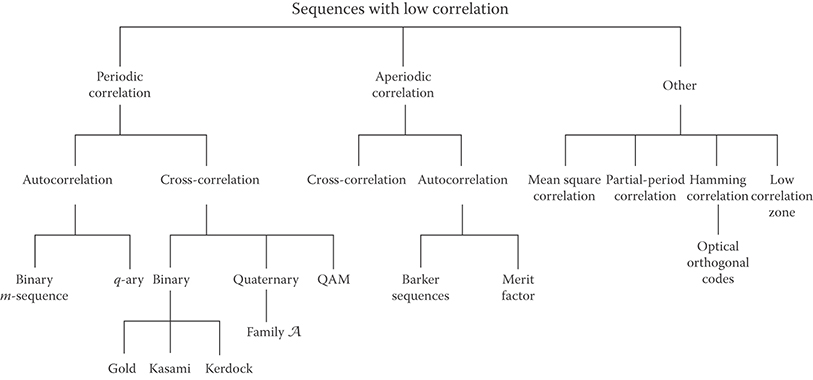
FIGURE 12.1 Overview of pseudonoise sequences.

Expanded tutorial discussions on pseudorandom sequences may be found in [9], [11], [12], [13, Chapter 21], [27], and [28, Chapter 5]. Sequence design related to peak-power control is covered in [19] while some recent advances in the area are covered in [10].

12.2 m Sequences

A binary {0,1} shift-register sequence {s(t)} is a sequence that satisfies a linear recurrence relation of the form

\sum_{i = 0}^{r} f_{i} s (t + i) = 0, for all t \geq 0 (12.1)

$\sum_{i = 0}^{r} f_{i} s (t + i) = 0, for all t \geq 0 (12.1)$

where r ≥ 1 is the degree of the recursion; the coefficients f_i belong to the field GF(2) = {0,1} where the leading coefficient f_r = 1. Thus, both sequences {a(t)} and {b(t)} appearing in Figure 12.2 are shift-register sequences.

Images

FIGURE 12.2 An example Gold sequence generator. Here, {a(t)} and {b(t)} are m sequences of length 7.

A sequence satisfying a recursion of the form in Equation 12.1 is said to have characteristic polynomial $f (x) = \sum_{i = 0}^{r} f_{i} x^{i}$ $f (x) = \sum_{i = 0}^{r} f_{i} x^{i}$ . Thus, {a(t)} and {b(t)} have characteristic polynomials given by f(x) = x³ + x + 1 and f(x) = x³ + x² + 1, respectively.

Since an r-bit binary shift register can assume a maximum of 2^r different states, it follows that every shift-register sequence {s(t)} is eventually periodic with period n ≤ 2^r, that is,

s (t) = s (t + n), for all t \geq N

$s (t) = s (t + n), for all t \geq N$

for some integer N. In fact, the maximum period of a shift-register sequence is 2^r – 1, since a shift register that enters the all-zero state will remain forever in that state. The upper shift register in Figure 12.2 when initialized with starting state 001 generates the periodic sequence {a(t)} given by

0010111 0010111 0010111 \dots (12.2)

$0010111 0010111 0010111 \dots (12.2)$

of period n = 7. It follows then that this shift register generates sequences of maximal period starting from any nonzero initial state.

An m sequence is simply a binary shift-register sequence having maximal period. For every r ≥ 1, m sequences are known to exist. The periodic autocorrelation function θ_s of a binary {0,1} sequence {s(t)} of period n is defined by

θ_{s} (τ) = \sum_{t = 0}^{n - 1} {(- 1)}^{s (t + τ) - s (t)}, 0 \leq τ \leq n - 1.

$θ_{s} (τ) = \sum_{t = 0}^{n - 1} {(- 1)}^{s (t + τ) - s (t)}, 0 \leq τ \leq n - 1.$

An m sequence of length n = 2^r – 1 has the following attributes: (1) Balance property: in each period of the m sequence there are 2^r−1 ones and 2^r−1 – 1 zeros. (2) Run property: every nonzero binary s-tuple, s ≤ r occurs 2^r−s times, the all-zero s-tuple occurs 2^r−s – 1 times. (3) Two-level autocorrelation function:

θ_{s} (τ) = {\begin{array}{l} n & if τ = 0 \\ - 1 & if τ \neq 0. \end{array} (12.3)

$θ_{s} (τ) = {\begin{array}{l} n & if τ = 0 \\ - 1 & if τ \neq 0. \end{array} (12.3)$

The first two properties follow immediately from the observation that every nonzero r-tuple occurs precisely once in each period of the m sequence. For the third property, consider the difference sequence {s(t + τ) – s(t)} for τ ≠ 0. This sequence satisfies the same recursion as the m sequence {s(t)} and is clearly not the all-zero sequence. It follows, therefore, that {s(t + τ)–s(t)} ≡ {s(t + τ′)} for some τ′, 0 ≤ τ′ ≤ n–1, that is, a different cyclic shift of the m sequence {s(t)}. The balance property of the sequence {s(t + τ′)} then gives us attribute 3. The m sequence {a(t)} in Equation 12.2 can be seen to have the three listed properties.

If {s(t)} is any sequence of period n and d is an integer, 1 ≤ d ≤ n, then the mapping {s(t)} → {s(dt)} is referred to as a decimation of {s(t)} by the integer d. If {s(t)} is an m sequence of period n = 2^r – 1 and d is an integer relatively prime to 2^r – 1, then the decimated sequence {s(dt)} clearly also has period n. Interestingly, it turns out that the sequence {s(dt)} is always also an m sequence of the same period. For example, when {a(t)} is the sequence in Equation 12.2, then

a (3 t) = 0011101 0011101 0011101 \dots (12.4)

$a (3 t) = 0011101 0011101 0011101 \dots (12.4)$

and

a (2 t) = 0111001 0111001 0111001 \dots . (12.5)

$a (2 t) = 0111001 0111001 0111001 \dots . (12.5)$

The sequence {a(3t)} is also an m sequence of period 7, since it satisfies the recursion

s (t + 3) + s (t + 2) + s (t) = 0 for all t

$s (t + 3) + s (t + 2) + s (t) = 0 for all t$

of degree r = 3. In fact, {a(3t)} is precisely the sequence labeled {b(t)} in Figure 12.2. The sequence {a(2t)} is simply a cyclically shifted version of {a(t)} itself; this property holds in general. If {s(t)} is any m sequence of period 2^r – 1, then {s(2t)} will always be a shifted version of the same m sequence. Clearly, the same is true for decimations by any power of 2.

Starting from an m sequence of period 2^r – 1, it turns out that one can generate all m sequences of the same period through decimations by integers d relatively prime to 2^r – 1. The set of integers d, 1 ≤ d ≤ 2^r – 1 satisfying (d,2^r – 1) = 1 forms a group under multiplication modulo 2^r – 1, with the powers {2ⁱ|0 ≤ i ≤ r – 1} of 2 forming a subgroup of order r. Since decimation by a power of 2 yields a shifted version of the same m sequence, it follows that the number of distinct m sequences of period 2^r – 1 is [φ(2^r – 1)/r], where φ(n) denotes the number of integers d, 1 ≤ d ≤ n, relatively prime to n. For example, when r = 3, there are just two cyclically distinct m sequences of period 7, and these are precisely the sequences {a(t)} and {b(t)} discussed in the preceding paragraph. The tables provided in [25] can be used to determine the characteristic polynomial of the various m sequences obtainable through the decimation of a single given m sequence. The classical reference on m sequences is [11].

If one obtains a sequence of some large length n by repeatedly tossing an unbiased coin, then such a sequence will very likely satisfy the balance, run, and autocorrelation properties of an m sequence of comparable length. For this reason, it is customary to regard the extent to which a given sequence possesses these properties as a measure of randomness of the sequence. Quite apart from this, in many applications such as signal synchronization and radar ranging, it is desirable to have sequences {s(t)} with low autocorrelation sidelobes, that is, |θ_s(τ)| is small for τ ≠ 0. Whereas m sequences are a prime example, there exist other methods of constructing binary sequences with low out-of-phase autocorrelation.

Sequences {s(t)} of period n having an autocorrelation function identical to that of an m sequence, that is, having θ_s satisfying Equation 12.3 correspond to well-studied combinatorial objects known as cyclic Hadamard difference sets. Known infinite families of such difference sets fall into three classes: (1) Singer and Gordon, Mills, and Welch (GMW), (2) quadratic residue, and (3) twin-prime difference sets. These correspond, respectively, to sequences of period n of the form n = 2^r – 1, r ≥ 1; n prime; and n = p(p + 2) with both p and p + 2 being prime in the last case. For a detailed treatment of cyclic difference sets, see [3].

Some 40 years after the appearance of the GMW construction, new and interesting cyclic Hadamard difference sets with Singer parameters were discovered in the late 1990s by several research groups. In 1998, Maschietti [21] constructed a new family of cyclic Hadamard difference sets that were based on the theory of hyperovals in finite projective geometry. Around the same time, several difference sets were postulated by No et al. in [23] based on the results of a numeric search and these led to a subsequent postulate by Dobbertin [8]. All postulates have now been confirmed to hold. The difference sets postulated by No et al. and Dobbertin were subsequently shown by Dillon [6] and Dillon and Dobbertin [7] to be examples of difference sets constructed by considering the image set, in a finite field with 2^m elements, of one of two mappings

\begin{array}{l} x \to {(x + 1)}^{d} + x^{d} + 1 & for d = 2^{2 k} - 2^{k} + 1 and \gcd (m, k) = 1 or \\ x \to {(x + 1)}^{d} + x^{d} & for d = 2^{2 k} - 2^{k} + 1 and 3 k \equiv 1 \mod (m) . \end{array}

$\begin{array}{l} x \to {(x + 1)}^{d} + x^{d} + 1 & for d = 2^{2 k} - 2^{k} + 1 and \gcd (m, k) = 1 or \\ x \to {(x + 1)}^{d} + x^{d} & for d = 2^{2 k} - 2^{k} + 1 and 3 k \equiv 1 \mod (m) . \end{array}$

The status at present is that all binary sequences of period 2ⁿ – 1 with ideal autocorrelation for n ≤ 10 can now be explained using known constructions.

12.3 The q-ary Sequences with Low Autocorrelation

As defined earlier, the autocorrelation of a binary {0,1} sequence {s(t)} leads to the computation of the inner product of an {–1, +1} sequence {(–1)^s(t)} with a cyclically shifted version {(–1)^s(t+τ)} of itself. The {–1, +1} sequence is transmitted as a phase shift by either 0° or 180° of a radio-frequency carrier, that is, using binary phase-shift keying (PSK) modulation. If the modulation is q-ary PSK, then one is led to consider sequences {s(t)} with symbols in the set $ℤ_{q}$ $ℤ_{q}$ , that is, the set of integers modulo q. The relevant autocorrelation function θ_s(τ) is now defined by

θ_{s} (τ) = \sum_{t = o}^{n - 1} ω^{s (t + τ) - s (t)},

$θ_{s} (τ) = \sum_{t = o}^{n - 1} ω^{s (t + τ) - s (t)},$

where n is the period of {s(t)} and ω is a complex primitive qth root of unity such as, for example, $ω = e^{i (2 π / q)}$ $ω = e^{i (2 π / q)}$ . It is possible to construct sequences {s(t)} over $ℤ_{q}$ $ℤ_{q}$ whose autocorrelation function satisfies

θ_{s} (τ) = {\begin{matrix} n & if τ = 0 \\ 0 & if τ \neq 0. \end{matrix}

$θ_{s} (τ) = {\begin{matrix} n & if τ = 0 \\ 0 & if τ \neq 0. \end{matrix}$

For obvious reasons, such sequences are said to have an ideal autocorrelation function.

We provide without proof two sample constructions. The sequences in the first construction are given by

s (t) = {\begin{matrix} t^{2} / 2 (\mod n) & when n is even \\ t (t + 1) / 2 (mod n) & when n is odd . \end{matrix}

$s (t) = {\begin{matrix} t^{2} / 2 (\mod n) & when n is even \\ t (t + 1) / 2 (mod n) & when n is odd . \end{matrix}$

Thus, this construction provides sequences with ideal autocorrelation for any period n. Note that the size q of the sequence symbol alphabet equals n when n is odd and 2n when n is even.

The second construction also provides sequences over $ℤ_{q}$ $ℤ_{q}$ of period n but requires that n be a perfect square. Let n = r² and let π be an arbitrary permutation of the elements in the subset {0,1,2,…,(r – 1)} of $ℤ_{n} :$ $ℤ_{n} :$ Let g be an arbitrary function defined on the subset {0,1,2,…,r – 1} of $ℤ_{n}$ $ℤ_{n}$ . Then, any sequence of the form

s (t) = r t_{1} π (t_{2}) + g (t_{2}) (\mod n),

$s (t) = r t_{1} π (t_{2}) + g (t_{2}) (\mod n),$

where t = rt₁ + t₂ with 0 ≤ t₁, t₂ ≤ r – 1 is the base-r decomposition of t, has an ideal autocorrelation function. When the alphabet size q equals or divides the period n of the sequence, ideal autocorrelation sequences also go by the name generalized bent functions. For details, see [17]. A different approach to the construction of ideal autocorrelation sequences and based on the Zak transform, is described in [1].

12.4 Families of Sequences with Low Cross-Correlation

Given two sequences {s₁(t)} and {s₂(t)} over $ℤ_{q}$ $ℤ_{q}$ of period n, their cross-correlation function θ_1,2(τ) is defined by

θ_{1, 2} (τ) = \sum_{t = o}^{n - 1} ω^{s_{1} (t + τ) - s_{2} (t)},

$θ_{1, 2} (τ) = \sum_{t = o}^{n - 1} ω^{s_{1} (t + τ) - s_{2} (t)},$

where ω is as before a primitive qth root of unity. The cross-correlation function is important in code-division multiple-access (CDMA) communication systems. Here, each user is assigned a distinct signature sequence and to minimize interference due to the other users, it is desirable that the signature sequences have pairwise, low values of cross-correlation function. To provide the system in addition with a self-synchronizing capability, it is desirable that the signature sequences have low values of the autocorrelation function as well.

Let $ℱ = {{s_{i} (t)} | 1 \leq i \leq M}$ $ℱ = {{s_{i} (t)} | 1 \leq i \leq M}$ be a family of M sequences {s_i(t)} over $ℤ_{q}$ $ℤ_{q}$ , each of period n. Let θ_i,j(τ) denote the cross-correlation between the ith and jth sequence at shift τ, that is,

θ_{i, j} (τ) = \sum_{t = o}^{n - 1} ω^{s_{i} (t + τ) - s_{j} (t)}, 0 \leq τ \leq n - 1 .

$θ_{i, j} (τ) = \sum_{t = o}^{n - 1} ω^{s_{i} (t + τ) - s_{j} (t)}, 0 \leq τ \leq n - 1 .$

The classical goal in sequence design for CDMA systems has been minimization of the parameter

θ_{\max} = \max {| θ_{i, j} (τ) | either i \neq j or τ \neq 0}

$θ_{\max} = \max {| θ_{i, j} (τ) | either i \neq j or τ \neq 0}$

for fixed n and M. It should be noted though that, in practice, because of data modulation the correlations that one runs into are typically of an aperiodic rather than a periodic nature (see Section 12.5). The problem of designing for low aperiodic correlation, however, is a more difficult one. A typical approach, therefore, has been to design based on periodic correlation, and then to analyze the resulting design for its aperiodic correlation properties. Again, in many practical systems, the mean square correlation properties are of greater interest than the worst-case correlation represented by a parameter such as θ_max. The mean square correlation is discussed in Section 12.6.2. Low correlation zone sequences, described in Section 12.6.3, are of interest when the CDMA system possesses approximate, but not perfect synchronism.

Bounds on the minimum possible value of θ_max for given period n, family size M, and alphabet size q are available that can be used to judge the merits of a particular sequence design. The most efficient bounds are those due to Welch, Sidelnikov, and Levenshtein; see [13]. In CDMA systems, there is greatest interest in designs in which the parameter θ_max is in the range $\sqrt{n} \leq θ_{\max} \leq 2 \sqrt{n}$ $\sqrt{n} \leq θ_{\max} \leq 2 \sqrt{n}$ . Accordingly, Table 12.1 uses the Welch, Sidelnikov, and Levenshtein bounds to provide an order-of-magnitude upper bound on the family size M for certain θ_max in the cited range.

Practical considerations dictate that q be small. The bit-oriented nature of electronic hardware makes it preferable to have q a power of 2. With this in mind, a description of some efficient sequence families having low auto- and cross-correlation values and alphabet sizes q = 2 and q = 4 are described below. Also included below is a description of a family of low-correlation sequences over the M²-quadrature amplitude modulation (QAM) alphabet for M = 2^m as this is an alphabet in common use in present-day communication systems. A discussion on the construction of families of ideal-autocorrelation q-ary sequences with low values of cross-correlation can be found in [1].

TABLE 12.1 Bounds on Family Size M for Given n, θ_max

θ_max	Upper Bound on M (q = 2)	Upper Bound on M (q > 2)
$\sqrt{n}$ $\sqrt{n}$	n/2	n
$\sqrt{2 n}$ $\sqrt{2 n}$	n	n²/2
$2 \sqrt{n}$ $2 \sqrt{n}$	3n²/10	n³/2

12.4.1 Gold and Kasami Sequences

Given the low autocorrelation sidelobes of an m sequence, it is natural to attempt to construct families of low correlation sequences starting from m sequences. Two of the better known constructions of this type are the families of Gold and Kasami sequences.

Let r be odd and d = 2^k + 1, where k, 1 ≤ k ≤ r – 1, is an integer satisfying (k, r) = 1. Let {s(t)} be a cyclic shift of an m sequence of period n = 2^r – 1 that satisfies $s (d t) \equiv 0$ $s (d t) \equiv 0$ and let $G$ $G$ be the Gold family of 2^r + 1 sequences given by

G = {s (t)} \cup {s (d t)} \cup {{s (t) + s (d [t + τ])} | 0 \leq τ \leq n - 1} .

$G = {s (t)} \cup {s (d t)} \cup {{s (t) + s (d [t + τ])} | 0 \leq τ \leq n - 1} .$

Then, each sequence in $G$ $G$ has period 2^r – 1 and the maximum-correlation parameter θ_max of $G$ $G$ satisfies

θ_{\max} \leq \sqrt{2^{r}} + 1.

$θ_{\max} \leq \sqrt{2^{r}} + 1.$

An application of the Sidelnikov bound coupled with the information that θ_max must be an odd integer yields that for the Family $G, θ_{\max}$ $G, θ_{\max}$ is as small as it can possibly be. In this sense, Family $G$ $G$ is an optimal family. We remark that these comments remain true even when d is replaced by the integer d = 2^2k – 2^k + 1 with the conditions on k remaining unchanged. The Gold family remains the best-known family of m sequences having low cross-correlation. Applications include the Navstar Global Positioning System whose signals are based on Gold sequences.

The family of Kasami sequences has a similar description. Let r = 2v and d = 2^v + 1. Let {s(t)} be a cyclic shift of an m sequence of period n = 2^r – 1 that satisfies $s (d t) \equiv 0$ $s (d t) \equiv 0$ , and consider the family of Kasami sequences given by

K = {s (t)} \cup {{s (t) + s (d [t + τ])} | 0 \leq τ \leq 2^{v} - 2} .

$K = {s (t)} \cup {{s (t) + s (d [t + τ])} | 0 \leq τ \leq 2^{v} - 2} .$

Then the Kasami family $K_{E}$ $K_{E}$ contains 2^v sequences of period 2^r – 1. It can be shown that in this case

θ_{\max} = 1 + 2^{v} .

$θ_{\max} = 1 + 2^{v} .$

This time an application of the Welch bound and the fact that θ_max is an integer shows that the Kasami family is optimal in terms of having the smallest possible value of θ_max for given n and M.

12.4.2 Quaternary Sequences

The entries in Table 12.1 suggest that nonbinary (i.e., q > 2) designs may be used for improved performance. A family of quaternary sequences that outperform the Gold and Kasami sequences is now discussed below.

Let f(x) be the characteristic polynomial of a binary m sequence of length 2^r – 1 for some integer r. The coefficients of f(x) are either 0 or 1. Now, regard f(x) as a polynomial over $ℤ_{4}$ $ℤ_{4}$ and form the product (–1)^rf(x)f(–x). This can be seen to be a polynomial in x². Define the polynomial g(x) of degree r by setting g(x²) = (–1)^rf(x)f(–x). Let $g (x) = \sum_{i = 0}^{r} g_{i} x^{i}$ $g (x) = \sum_{i = 0}^{r} g_{i} x^{i}$ and consider the set of all quaternary sequences {a(t)} satisfying the recursion $\sum_{i = 0}^{r} g_{i} a (t + i) = 0 (mod 4)$ $\sum_{i = 0}^{r} g_{i} a (t + i) = 0 (mod 4)$ for all t.

It turns out that with the exception of the all-zero sequence, all of the sequences generated in this way have period 2^r – 1. Thus, the recursion generates a Family A of 2^r + 1 cyclically distinct quaternary sequences. Closer study reveals that the maximum correlation parameter θ_max of this family satisfies $θ_{max} \leq 1 + \sqrt{2^{r}}$ $θ_{max} \leq 1 + \sqrt{2^{r}}$ . Thus, in comparison with the family of Gold sequences, the Family $A$ $A$ offers a lower value of θ_max (by a factor of $\sqrt{2}$ $\sqrt{2}$ ) for the same family size. In comparison with the set of Kasami sequences, it offers a much larger family size for the same bound on θ_max. Family $A$ $A$ sequences are discussed in [13] and in the references contained therein.

Images

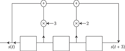
FIGURE 12.3 Shift register that generates family $A$ $A$ quaternary sequences {s(t)} of period 7.

We illustrate with an example. Let f(x) = x³ + x + 1 be the characteristic polynomial of the m sequence {a(t)} in Equation 12.1. Then, over $ℤ_{4}$ $ℤ_{4}$

g (x^{2}) = {(- 1)}^{3} f (x) f (- x) = x^{6} + 2 x^{4} + x^{2} + 3

$g (x^{2}) = {(- 1)}^{3} f (x) f (- x) = x^{6} + 2 x^{4} + x^{2} + 3$

so that g(x) = x³ + 2x² + x + 3. Thus, the sequences in Family $A$ $A$ are generated by the recursion s(t + 3) + 2s(t + 2) + s(t + 1) + 3s(t) = 0 (mod 4). The corresponding shift register is shown in Figure 12.3.

By varying initial conditions, this shift register can be made to generate nine cyclically distinct sequences, each of length 7. In this case, $θ_{\max} \leq 1 + \sqrt{8}$ $θ_{\max} \leq 1 + \sqrt{8}$ .

12.4.3 Binary Kerdock Sequences

The Gold and Kasami families of sequences are closely related to binary linear cyclic codes. It is known in coding theory, that there exists nonlinear binary codes the performance of which exceeds that of the best-possible linear code. Surprisingly, some of these examples come from binary codes, which are images of linear quaternary (q = 4) codes under the Gray map: 0 → 00, 1 → 01, 2 → 11, 3 → 10. A prime example of this is the Kerdock code, which has been shown to be the Gray image of a quaternary linear code. Thus, it is not surprising that the Kerdock code yields binary sequences, which we term as Kerdock sequences here, which improve upon the performance of the family of Kasami sequences.

The Kerdock sequences may be constructed as follows: let f(x) be the characteristic polynomial of an m sequence of period 2^r – 1, r odd. As before, regarding f(x) as a polynomial over $ℤ_{4}$ $ℤ_{4}$ (which happens to have {0, 1} coefficients), let the polynomial g(x) over $ℤ_{4}$ $ℤ_{4}$ be defined via g(x²) = –f(x)f(–x). Thus, g(x) is the characteristic polynomial of a Family $A$ $A$ sequence set of period 2^r – 1. Set $h (x) = - g (- x) = \sum_{i = 0}^{r} h_{i} x^{i}$ $h (x) = - g (- x) = \sum_{i = 0}^{r} h_{i} x^{i}$ , and let S be the set of all $ℤ_{4}$ $ℤ_{4}$ sequences satisfying the recursion $\sum_{i = 0}^{r} h_{i} s (t + i) = 0$ $\sum_{i = 0}^{r} h_{i} s (t + i) = 0$ . Then, Family S contains 4^r-distinct sequences corresponding to all possible distinct initializations of the shift register.

Let T denote a subset of S of size 2^r consisting of those sequences corresponding to initializations of the shift register only using the symbols 0 and 2 in $ℤ_{4}$ $ℤ_{4}$ . Then the set S – T of size 4^r – 2^r contains a set $U$ $U$ of 2^r−1 cyclically distinct sequences each of period 2(2^r – 1). Given $x = a + 2 b \in ℤ_{4}$ $x = a + 2 b \in ℤ_{4}$ with a,b ∈ {0,1}, let µ denote the most significant bit (MSB) map µ(x) = b. Let $K_{E}$ $K_{E}$ denote the family of 2^r−1 binary sequences obtained by applying the map µ to each sequence in $U$ $U$ . It turns out that each sequence in $U$ $U$ also has period 2(2^r – 1) and that, furthermore, for the Family $K_{E}$ $K_{E}$ , $θ_{\max} \leq 2 + \sqrt{2^{r + 1}}$ $θ_{\max} \leq 2 + \sqrt{2^{r + 1}}$ . Thus, $K_{E}$ $K_{E}$ is a much larger family than the Kasami family, while having almost exactly the same value of θ_max.

For example, taking r = 3 and f(x) = x³ + x + 1, we have from the previous Family $A$ $A$ example that g(x) = x³ + 2x² + x + 3, so that h(x) = –g(–x) = x³ + 2x² + x + 1. Applying the MSB map to the head of the shift register, and discarding initializations of the shift register involving only 0’s and 2’s yields a family of four cyclically distinct binary sequences of period 14. Kerdock sequences are discussed in [13] and in the references contained therein.

12.4.3.1 QAM Sequences

For M an even integer, the M²-QAM alphabet is given by

{a + i b | - (M - 1) \leq a, b \leq (M - 1), a, b odd}

${a + i b | - (M - 1) \leq a, b \leq (M - 1), a, b odd}$

When $M = 2^{m}, m \geq 2$ $M = 2^{m}, m \geq 2$ , this alphabet can alternately be represented in the form:

{\sqrt{2} i \sum_{k = 0}^{m - 1} 2^{k} i^{a_{k}} | a_{k} \in ℤ_{4}} .

${\sqrt{2} i \sum_{k = 0}^{m - 1} 2^{k} i^{a_{k}} | a_{k} \in ℤ_{4}} .$

The connection with $ℤ_{4}$ $ℤ_{4}$ suggests the use of quaternary sequences in the construction of low-correlation QAM sequences and an example construction over the 16-QAM alphabet is presented below. Sequences over the QAM alphabet are of interest as QAM is a signaling alphabet that is commonly employed in practice, and additionally, in the context of a CDMA system, a QAM sequence can potentially be made to carry a greater amount of data. Let the 2^r sequences in Family $A$ $A$ of period $N : = 2^{r} - 1$ $N : = 2^{r} - 1$ be partitioned into $2^{r}$ $2^{r}$ disjoint pairs ${{a_{i} (t), b_{i} (t)} | 1 \leq i \leq 2^{r}}$ ${{a_{i} (t), b_{i} (t)} | 1 \leq i \leq 2^{r}}$ . Then, a Family $ℂ ℚ$ $ℂ ℚ$ (for canonical QAM family) of 16-QAM sequences may be described as follows:

ℂ ℚ = {s_{i} (t) | 1 \leq i \leq 2^{r}}

$ℂ ℚ = {s_{i} (t) | 1 \leq i \leq 2^{r}}$

where

s_{i} (t) = \sqrt{2} i (i^{a_{i} (t)} + 2 i^{b_{i} (t)})

$s_{i} (t) = \sqrt{2} i (i^{a_{i} (t)} + 2 i^{b_{i} (t)})$

For the Family $ℂ ℚ$ $ℂ ℚ$ , it can be shown that the maximum correlation parameter $θ_{max}$ $θ_{max}$ , after normalization, satisfies

θ_{max} \leq 1.8 \sqrt{N} .

$θ_{max} \leq 1.8 \sqrt{N} .$

Normalization is carried out by dividing each correlation value $θ_{i, j} (τ)$ $θ_{i, j} (τ)$ by the factor 10 because each sequence $s_{i} (t)$ $s_{i} (t)$ has energy

\sum_{t = 0}^{2^{r} - 2} {| s_{i} (t) |}^{2} \approx 10 N,

$\sum_{t = 0}^{2^{r} - 2} {| s_{i} (t) |}^{2} \approx 10 N,$

when one neglects terms of order $\sqrt{N}$ $\sqrt{N}$ , whereas, in comparison, each q-ary sequences of period N has energy N. To convey data, the actual signal transmitted by the user is then given by

s_{i} (t, κ) = \sqrt{2} i (i^{a_{i} (t) + κ_{a}} + 2 i^{b_{i} (t) + κ_{b}}),

$s_{i} (t, κ) = \sqrt{2} i (i^{a_{i} (t) + κ_{a}} + 2 i^{b_{i} (t) + κ_{b}}),$

where $κ_{a}, κ_{b} lie in ℤ_{4}$ $κ_{a}, κ_{b} lie in ℤ_{4}$ and represent data, so that one period of the sequence carries 4 bits of data. Further details including improved constructions and generalization to the general $2^{2 m}$ $2^{2 m}$ -QAM constellation alphabet can be found in [2], [5], and [10].

12.5 Aperiodic Correlation

Let {x(t)} and {y(t)} be complex-valued sequences of length (or period) n, not necessarily distinct. Their aperiodic correlation values {ρ_x,y(τ)| – (n – 1) ≤ τ ≤ n – 1} are given by

ρ_{x, y} (τ) = \sum_{t = \max {0, - τ}}^{\min {n - 1, n - 1 - τ}} x (t + τ) y^{*} (t),

$ρ_{x, y} (τ) = \sum_{t = \max {0, - τ}}^{\min {n - 1, n - 1 - τ}} x (t + τ) y^{*} (t),$

where y*(t) denotes the complex conjugate of y(t). When x ≡ y, we will abbreviate and write ρ_x in place of ρ_x,y. The sequences described next are perhaps the most famous example of sequences with low-aperiodic autocorrelation values.

12.5.1 Barker Sequences

A binary {–1, +1} sequence {s(t)} of length n is said to be a Barker sequence [3] if the aperiodic autocorrelation values ρ_s(τ) satisfy |ρ_s(τ)| ≤ 1 for all τ, –(n – 1) ≤ τ ≤ n – 1. The Barker property is preserved under the following transformations:

s (t) \to - s (t), s (t) \to {(- 1)}^{t} s (t) and s (t) \to s (n - 1 - t)

$s (t) \to - s (t), s (t) \to {(- 1)}^{t} s (t) and s (t) \to s (n - 1 - t)$

as well as under compositions of the preceding transformations. Only the following Barker sequences are known:

\begin{matrix} n = 2 + + \\ n = 3 + + - \\ n = 4 + + + - \\ n = 5 + + + - + \\ n = 7 + + + - - + - \\ n = 11 + + + - - - + - - + - \\ n = 13 + + + + + - - + + - + - +, \end{matrix}

$\begin{matrix} n = 2 + + \\ n = 3 + + - \\ n = 4 + + + - \\ n = 5 + + + - + \\ n = 7 + + + - - + - \\ n = 11 + + + - - - + - - + - \\ n = 13 + + + + + - - + + - + - +, \end{matrix}$

where + denotes +1 and − denotes –1, apart from sequences that are generated from these via the transformations already discussed. It is known that if any other Barker sequence exists, it must have length n > 1,898,884, that is a multiple of 4.

An upper bound on the maximum out-of-phase aperiodic autocorrelation of an m sequence can be found in [26].

12.5.2 Sequences with High Merit Factor

The merit factor F of a {–1, +1} sequence {s(t)} is defined by

F = \frac{n^{2}}{2 \sum_{τ = 1}^{n - 1} ρ_{s}^{2} (τ)} .

$F = \frac{n^{2}}{2 \sum_{τ = 1}^{n - 1} ρ_{s}^{2} (τ)} .$

Since ρ_s(τ) = ρ_s(–τ) for 1 ≤ |τ| ≤ n – 1 and ρ_s(0) = n, the factor F may be regarded as the ratio of the square of the in-phase autocorrelation, to the sum of the squares of the out-of-phase aperiodic autocorrelation values. Thus, the merit factor is one measure of the aperiodic autocorrelation properties of a binary {–1, +1} sequence. It is also closely connected with the signal to self-generated noise ratio of a communication system in which coded pulses are transmitted and received.

Let F_n denote the largest merit factor of any binary {–1, +1} sequence of length n. For example, at length n = 13, the Barker sequence of length 13 has a merit factor F = F₁₃ = 14.08. Assuming a certain ergodicity postulate it was established by Golay that lim_n→∞ F_n = 12.32. Exhaustive computer searches carried out for n ≤ 40 have revealed the following.

For 1 ≤ n ≤ 40, n ≠ 11,13.
F₁₁ = 12.1, F₁₃ = 14.08, 3.3 ≤ F_n ≤ 9.85.

The value F₁₁ is also achieved by a Barker sequence. From partial searches, for lengths up to 117, the highest known merit factor is between 8 and 9.56; for lengths from 118 to 200, the best-known factor is close to 6. For lengths >200, statistical search methods have failed to yield a sequence having merit factor exceeding 5.

An offset sequence is one in which a fraction θ of the elements of a sequence of length n are chopped off at one end and appended to the other end, that is, an offset sequence is a cyclic shift of the original sequence by nθ symbols. It turns out that the asymptotic merit factor of m sequences is equal to 3 and is independent of the particular offset of the m sequence. There exist offsets of sequences associated with quadratic-residue and twin-prime difference sets that achieve a larger merit factor of 6. Details may be found in [14,15].

In 1999, Kirilusha and Narayanaswamy made the interesting observation that when one started with a sequence from a family with asymptotic merit factor 6 and appended the initial part of the sequence to the sequence, the resultant sequence was found through numerical experiments, to often have a merit factor strictly greater than 6. Following up on this approach, [4] and [16] were able to construct sequence families whose asymptotic merit factor was numerically observed to approach a value greater than 6.34. An analytical proof of the same however, is still lacking. Their constructions were based on cyclic shifts S_r of a Legendre sequence S by a fraction r of the period to which is then appended, a fraction t, 0 < t < 1, of the initial portion of S_r. There is extensive numerical evidence to indicate that for large n, the merit factor of the new sequence is greater than 6.2 when r = 0.25 and t ≈ 0.03 and further that when r ≈ 0.22 and t ≈ 0.06, the merit factor of the new sequence is greater than 6.34. Providing an analytical proof of these properties remains a challenging open problem. There is of course beyond this, the larger open question of determining the largest possible asymptotic merit factor F_n of any binary sequence.

12.5.3 Sequences with Low Aperiodic Cross-Correlation

If {u(t)} and {v(t)} are sequences of length 2n – 1 defined by

u (t) = {\begin{array}{l} x (t) & if 0 \leq t \leq n - 1 \\ 0 & if n \leq t \leq 2 n - 2 \end{array}

$u (t) = {\begin{array}{l} x (t) & if 0 \leq t \leq n - 1 \\ 0 & if n \leq t \leq 2 n - 2 \end{array}$

and

υ (t) = {\begin{array}{l} y (t) & if 0 \leq t \leq n - 1 \\ 0 & if n \leq t \leq 2 n - 2 \end{array},

$υ (t) = {\begin{array}{l} y (t) & if 0 \leq t \leq n - 1 \\ 0 & if n \leq t \leq 2 n - 2 \end{array},$

then

{ρ_{x, y} (τ) | - (n - 1) \leq τ \leq n - 1} = {θ_{u, v} (τ) | 0 \leq τ \leq 2 n - 2} . (12.6)

${ρ_{x, y} (τ) | - (n - 1) \leq τ \leq n - 1} = {θ_{u, v} (τ) | 0 \leq τ \leq 2 n - 2} . (12.6)$

Given a collection

U = {{x_{i} (t)} | 1 \leq i \leq M}

$U = {{x_{i} (t)} | 1 \leq i \leq M}$

of sequences of length n over $ℤ_{q}$ $ℤ_{q}$ , let us define

ρ_{\max} = \max {| ρ_{a, b} (τ) | | a, b \in U, either a \neq b or τ \neq 0},

$ρ_{\max} = \max {| ρ_{a, b} (τ) | | a, b \in U, either a \neq b or τ \neq 0},$

It is clear from Equation 12.6 how bounds on the periodic correlation parameter θ_max can be adapted to give bounds on ρ_max. Translation of the Welch bound (mentioned earlier in Section 12.4) gives that for every integer k ≥ 1,

ρ_{\max}^{2 k} \geq (\frac{n^{2 k}}{M (2 n - 1) - 1}) {\frac{M (2 n - 1)}{(\begin{matrix} 2 n + k - 2 \\ k \end{matrix})} - 1} .

$ρ_{\max}^{2 k} \geq (\frac{n^{2 k}}{M (2 n - 1) - 1}) {\frac{M (2 n - 1)}{(\begin{matrix} 2 n + k - 2 \\ k \end{matrix})} - 1} .$

Setting k = 1 in the preceding bound gives

ρ_{\max} \geq n \sqrt{\frac{M - 1}{M (2 n - 1) - 1}} . (12.7)

$ρ_{\max} \geq n \sqrt{\frac{M - 1}{M (2 n - 1) - 1}} . (12.7)$

Thus, for fixed M and large n, Welch's bound gives

ρ_{\max} \geq O (n^{1 / 2}) .

$ρ_{\max} \geq O (n^{1 / 2}) .$

There exist sequence families which asymptotically achieve $ρ_{\max} \approx O (n^{1 / 2})$ $ρ_{\max} \approx O (n^{1 / 2})$ [22].

12.6 Other Correlation Measures

12.6.1 Partial-Period Correlation

The partial-period (p-p) correlation between the sequences {u(t)} and {v(t)} is the collection {Δ_u,v(l,τ,t₀)|1 ≤ l ≤ n, 0 ≤ τ ≤ n – 1, 0 ≤ t₀ ≤ n – 1} of inner products

Δ_{u, v} (l, τ, t_{0}) = \sum_{t = t_{0}}^{t_{0} + l - 1} u (t + τ) v^{*} (t),

$Δ_{u, v} (l, τ, t_{0}) = \sum_{t = t_{0}}^{t_{0} + l - 1} u (t + τ) v^{*} (t),$

where l is the length of the partial period and the sum t + τ is again computed modulo n. In direct-sequence CDMA systems, the pseudorandom signature sequences used by the various users are often very long for reasons of data security. In such situations, to minimize receiver hardware complexity, correlation over a partial period of the signature sequence is often used to demodulate data as well as to achieve synchronization. For this reason, the p-p correlation properties of a sequence are of interest.

Researchers have attempted to determine the moments of the p-p correlation. Here, the main tool is the application of the Pless power-moment identities of coding theory [20]. The identities often allow the first and second p-p correlation moments to be completely determined. For example, this is true in the case of m sequences (the remaining moments turn out to depend upon the specific characteristic polynomial of the m sequence). Further details may be found in [28].

12.6.2 Mean Square Correlation

Frequently in practice, there is a greater interest in the mean-square correlation distribution of a sequence family than in the parameter θ_max. Quite often in sequence design, the sequence family is derived from a linear, binary cyclic code of length n by picking a set of cyclically distinct sequences of period n. The families of Gold and Kasami sequences are so constructed. In this case, as pointed out by Massey, the mean square correlation of the family can be shown to be either optimum or close to optimum, under certain easily satisfied conditions, imposed on the minimum distance of the dual code. A similar situation holds even when the sequence family does not come from a linear cyclic code. In this sense, mean square correlation is not a very discriminating measure of the correlation properties of a family of sequences. More details may be found in [13].

12.6.3 Low-Correlation Zone Sequences

For the case when there is approximate, but not perfect synchronism present in a CDMA communication system, there is interest in the design of families of sequences whose auto- and cross-correlations are small for small values of relative time shift [18]. In this context, a low correlation zone (LCZ) sequence family ${s_{i} (t)}_{i = 1}^{M}$ ${s_{i} (t)}_{i = 1}^{M}$ is defined as one in which the nontrivial auto- and cross-correlation values are small (typically 0 or −1) for small values of the time-shift parameter τ, that is,

| θ_{i, j} (τ) | \leq δ for | ​ τ | < L, i \neq j, and for 1 \leq | ​ τ ​ | < L, when i = j .

$| θ_{i, j} (τ) | \leq δ for | τ | < L, i \neq j, and for 1 \leq | τ | < L, when i = j .$

Four parameters (N,M,L,δ) characterize an LCZ sequence family, namely, the size M of the family, the common period N of each sequence in the family, the time duration L of the low correlation zone, and the upper bound δ on correlation magnitudes within the low correlation zone. The size M of an (N,M,L,δ) LCZ sequence family is upper bounded [29] by

M L - 1 \leq \frac{N - 1}{1 - \frac{δ^{2}}{N}} . (12.8)

$M L - 1 \leq \frac{N - 1}{1 - \frac{δ^{2}}{N}} . (12.8)$

For more details, the reader is referred to the overview in [10] and to the references cited therein.

12.6.4 Optical Orthogonal Codes

Given a pair of {0,1} sequences {s₁(t)} and {s₂(t)} each having period n, we define the Hamming correlation function θ₁₂(τ), 0 ≤ τ ≤ n – 1, by

θ_{12} (τ) = \sum_{t = 0}^{n - 1} s_{1} (t + τ) s_{2} (t) .

$θ_{12} (τ) = \sum_{t = 0}^{n - 1} s_{1} (t + τ) s_{2} (t) .$

Such correlations are of interest, for instance, in optical communication systems where the 1’s and 0’s in a sequence correspond to the presence or absence of pulses of transmitted light.

An (n,w,λ) optical orthogonal code (OOC) is a Family $ℱ = {{s_{i} (t)} | i = 1, 2, \dots, M}$ $ℱ = {{s_{i} (t)} | i = 1, 2, \dots, M}$ , of M{0,1} sequences of period n, constant Hamming weight w, where w is an integer lying between 1 and n – 1 satisfying θ_ij(τ) ≤ λ whenever either i ≠ j or τ ≠ 0.

Note that the Hamming distance d_a_,b between a period of the corresponding codewords {a(t)}, {b(t)}, 0 ≤ t ≤ n – 1 in an (n,w,λ) OOC having Hamming correlation ρ, 0 ≤ ρ ≤ λ, is given by d_a,b = 2(w – ρ), and, thus, OOCs are closely related to constant-weight error correcting codes. Given an (n,w,λ) OOC, by enlarging the OOC to include every cyclic shift of each sequence in the code, one obtains a constant-weight, minimum-distance d_min ≥ 2(w – λ) code. Conversely, given a constant-weight cyclic code of length n, weight w, and minimum distance d_min, one can derive an (n,w,λ) OOC code with λ ≤ w – d_min/2 by partitioning the code into cyclic equivalence classes and then picking precisely one representative from each equivalence class of size n.

By making use of this connection, one can derive bounds on the size of an OOC from known bounds on the size of constant-weight codes. The bound given next follows directly from the Johnson bound for constant weight codes [20]. The number M(n,w,λ) of codewords in a (n,w,λ) OOC satisfies

M (n, w, λ) \leq \frac{1}{w} ⌊ \frac{n - 1}{w - 1} \dots ⌊ \frac{n - λ + 1}{w - λ + 1} ⌊ \frac{n - λ}{w - λ} ⌋ ⌋ \dots ⌋ . (12.9)

$M (n, w, λ) \leq \frac{1}{w} ⌊ \frac{n - 1}{w - 1} \dots ⌊ \frac{n - λ + 1}{w - λ + 1} ⌊ \frac{n - λ}{w - λ} ⌋ ⌋ \dots ⌋ . (12.9)$

An OOC code that achieves the Johnson bound is said to be optimal. A family ${ℱ_{n}}$ ${ℱ_{n}}$ of OOCs indexed by the parameter n and arising from a common construction is said to be asymptotically optimum if

\lim_{n \to \infty} \frac{| ℱ_{n} |}{M (n, w, λ)} = 1.

$\lim_{n \to \infty} \frac{| ℱ_{n} |}{M (n, w, λ)} = 1.$

Constructions for OOCs are available for the cases when λ = 1 and λ = 2. For larger values of λ, there exist constructions which are asymptotically optimum. Further details may be found in [13].

2-D OOC: The OOC discussed above correspond to sequences of pulses of a single beam of monochromatic light. The advent of wavelength-division multiplexing has made it possible to design low-correlation optical signals that are spread across both wavelength and time. While such signals are often called wavelength-time hopping codes or multiple-wavelength codes, we will refer to these codes as two-dimensional OOCs (2-D OOCs). A 2-D (Λ × T,ω,κ) OOC C is a family of {0,1} (Λ × T) arrays of constant Hamming weight ω. Every pair {A,B} of arrays in C is required to satisfy

\sum_{λ = 1}^{Λ} \sum_{t = 0}^{T - 1} A (λ, t) B (λ, t \oplus_{T} τ) \leq κ, (12.10)

$\sum_{λ = 1}^{Λ} \sum_{t = 0}^{T - 1} A (λ, t) B (λ, t \oplus_{T} τ) \leq κ, (12.10)$

where either A ≠ B or τ ≠ 0. We will refer to κ as the maximum collision parameter (MCP) if κ ≥ 0 is the smallest integer for which Equation 12.10 holds. Note that asynchronism is present here only along the time axis. As in the 1-D case, in a 2-D optical CDMA system, each user is assigned a distinct 2-D OOC and when the particular user wishes to send either a 1 or a 0, the user either transmits or else does not transmit the user's code sequence, respectively. Given a parameter set, let φ(Λ × T,ω,κ) denote the largest possible cardinality of a 2-D OOC having these parameters. The analog of the Johnson bound for 2-D OOC is given by

ϕ (Λ \times T, ω, k) \leq ⌊ \frac{Λ}{ω} ⌊ \frac{Λ T - 1}{ω - 1} \dots ⌊ \frac{Λ T - κ}{ω - κ} ⌋ ⌋ ⌋ . (12.11)

$ϕ (Λ \times T, ω, k) \leq ⌊ \frac{Λ}{ω} ⌊ \frac{Λ T - 1}{ω - 1} \dots ⌊ \frac{Λ T - κ}{ω - κ} ⌋ ⌋ ⌋ . (12.11)$

The parameters n in the case of a 1-D OOC and the parameter T in the case of a 2-D OOC represent the multiplicative factor by which the pulse rate in the optical communication system has to be raised. Comparing Equation 12.11 with Equation 12.9, we see that for the same family size φ, the value of T in Equation 12.11 is significantly smaller than the value of n in Equation 12.9 and this is an important advantage enjoyed by a 2-D OOC. For details and constructions of 2-D OOC, the reader is referred to [24] and [30].

References

1. An M., Brodzik A.K., and Tolimieri R. Ideal Sequence Design in Time-Frequency Space: Applications to Radar, Sonar and Communication Systems, Birkhauser, Boston, 2009.

2. Anand M. and Kumar P.V. Low-correlation sequences over the QAM constellation, IEEE Transactions on Information Theory, IT-54, 791–810, 2008.

3. Baumert L.D. Cyclic Difference Sets, Lecture Notes in Mathematics, Vol. 182, Springer–Verlag, New York, 1971.

4. Borwein P., Choi K.-K.S., and Jedwab J. Binary sequences with merit factor greater than 6.34, IEEE Transactions on Information Theory, IT-50, 3234–3249, 2004.

5. Boztas S. CDMA over QAM and other arbitrary energy constellations, IEEE International Conference on Communication Systems, 2, 21.7.1–21.7.5, 1996.

6. Dillon J. Multiplicative difference sets via additive characters, Designs Codes and Cryptography, 17, 225–235, 1999.

7. Dillon J. and Dobbertin H. New cyclic difference sets with Singer parameters, Finite Fields and Their Applications, 10, 342–389, 2004.

8. Dobbertin H. Kasami power functions, permutation polynomials and cyclic difference sets, In Difference Sets, Sequences and Their Correlation Properties (eds.) A. Pott pp. 133–158, The Netherlands, Kluwer Academic Publishers, 1999.

9. Fan P. and Darnell M. Sequence Design for Communications Applications, John Wiley & Sons, London, 1996.

10. Garg G., Helleseth T., and Kumar P.V. Recent advances in low-correlation sequences, In New Directions in Wireless Communications Research (ed.) V. Tarokh, Springer, Berlin, 2009.

11. Golomb S.W. Shift Register Sequences, Aegean Park Press, San Francisco, CA, 1982.

12. Golomb S.W. and Gong G. Signal Design for Good Correlation: For Wireless Communication, Cryptography, and Radar, Cambridge University Press, New York, 2005.

13. Helleseth T. and Kumar P.V. Sequences with low correlation. In Handbook of Coding Theory (eds.) V.S. Pless and W.C. Huffman, Elsevier Science Publishers, Amsterdam, 1998.

14. Jedwab J. A survey of the merit factor problem for binary sequences, Proceedings of Sequences and Their Applications, 3486, 30–55, 2004.

15. Jensen J.M., Jensen H.E., and Høholdt T. The merit factor of binary sequences related to difference sets, IEEE Transactions on Information Theory, IT-37, 617–626, 1991.

16. Kristiansen R.A. and Parker M.G. Binary sequences with merit factor >6.3, IEEE Transactions on Information Theory, IT-50, 3385–3389, 2004.

17. Kumar P.V., Scholtz R.A., and Welch L.R. Generalized bent functions and their properties, Journal of Combinatorial Theory Series A., 40, 90–107, 1985.

18. Long B., Zhang P., and Hu J. A generalized QS-CDMA system and the design of new spreading codes, IEEE Transactions on Vehicular Technology, 47, 1268–1275, 1998.

19. Litsyn S. Peak Power Control in Multicarrier Communications, Cambridge University Press, New York, 2007.

20. MacWilliams F.J. and Sloane N.J.A. The Theory of Error-Correcting Codes, North-Holland, Amsterdam, 1977.

21. Maschietti A. Difference sets and hyperovals, Designs, Codes and Cryptography, 14, 89–98, 1998.

22. Mow W.H. On McEliece's open problem on minimax aperiodic correlation, Proceedings of the IEEE International Symposium on Information Theory, 75, 1994.

23. No J.-S., Golomb S.W., Gong G., Lee H.-K., and Gaal P. Binary pseudorandom sequences of period 2ⁿ – 1 with ideal autocorrelation properties, IEEE Transactions on Information Theory, IT-44, 814–817, 1998.

24. Omrani R. and Kumar P.V. Improved constructions and bounds for 2-D optical orthogonal codes, Proceedings of the IEEE International Symposium on Information Theory, 127–131, 2005.

25. Peterson W.W. and Weldon E.J., Jr. Error-Correcting Codes, 2nd ed., MIT Press, Cambridge, MA, 1972.

26. Sarwate D.V. An upper bound on the aperiodic autocorrelation function for a maximal-length sequence. IEEE Transactions on Information Theory, IT-30, 685–687, 1984.

27. Sarwate D.V. and Pursley M.B. Crosscorrelation properties of pseudorandom and related sequences, Proceedings of the IEEE, 68, 593–619, 1980.

28. Simon M.K., Omura J.K., Scholtz R.A., and Levitt B.K. Spread Spectrum Communications Handbook, revised ed., McGraw Hill, New York, 1994.

29. Tang X.H., Fan P.Z., and Matsufuji S. Lower bounds on correlation of spreading sequence set with low or zero correlation zone, Electronics Letters, 36, 551–552, 2000.

30. Yang G.C. and Kwong W.C. Two-dimensional spatial signature patterns, IEEE Transactions on Communications, 44, 184–191, 1996.

Table of Contents for
12 Pseudonoise Sequences

12

Pseudonoise Sequences

12.1 Introduction

12.2 m Sequences

12.3 The q-ary Sequences with Low Autocorrelation

12.4 Families of Sequences with Low Cross-Correlation

12.4.1 Gold and Kasami Sequences

12.4.2 Quaternary Sequences

12.4.3 Binary Kerdock Sequences

12.4.3.1 QAM Sequences

12.5 Aperiodic Correlation

12.5.1 Barker Sequences

12.5.2 Sequences with High Merit Factor

12.5.3 Sequences with Low Aperiodic Cross-Correlation

12.6 Other Correlation Measures

12.6.1 Partial-Period Correlation

12.6.2 Mean Square Correlation

12.6.3 Low-Correlation Zone Sequences

12.6.4 Optical Orthogonal Codes

References

Further Reading

Table of Contents for 12 Pseudonoise Sequences

Create new playlist

Sign In

Sign Up

12

12.4.3.1 QAM Sequences

Table of Contents for
12 Pseudonoise Sequences