
29
Video Compression
Do-Kyoung Kwon, Madhukar Budagavi, Vivienne Sze and Woo-Shik Kim
Digital Video and Need for Compression
Basic Video Coding Architecture
Profile Information and Performance Analysis
Stereo 3D Video Coding via H.264/AVC SEI Messages
29.5 High-Efficiency Video Coding
29.1 Introduction
Video compression has been a key enabling technology for a variety of consumer electronics devices and applications such as camera phones, DVD players, personal media players, digital camcorders, streaming video, video conferencing, and etc. This chapter provides an overview of video compression basics and video coding standards developed by ITU-T and ISO/IEC MPEG.
Video sequences contain a lot of redundancies and removing these redundancies is the fundamental objective of video compression. There are several different types of redundancies that exist in video sequences and techniques for removing them are presented first in this section. Early video coding standards including H.261, MPEG-1/2, H.263, and MPEG-4 are briefly introduced as well. Sections 29.2, 29.3, and 29.4 provide an overview of H.264/AVC (advanced video coding), the scalable extensions of H.264/AVC, and the multiview extension of H.264/AVC, respectively. Finally, high-efficiency video coding (HEVC), which is the next-generation video coding standard currently being developed, is briefly introduced in Section 29.5.
29.1.1 Digital Video and Need for Compression
Digital video data consist of a series of images captured using a camera or artificially generated (e.g., computer-generated movies). Figure 29.1a shows four images of a color video sequence captured at 30 frames per second (fps). Each image of color video consists of a luminance (also referred to as luma and denoted by Y) component and two chrominance components (also referred to as chroma and denoted by U and V). Since the human eye is more sensitive to luma than chroma, the chroma components are typically subsampled to lower the data rate. Figure 29.1b shows YUV 4:2:0 format image where the U and V chroma components are quarter the size of luma component. Consumer video is predominantly in the 4:2:0 format with 8 bits per pixel. Higher chroma resolution (no chroma subsampling) and higher bit depth (10-bits or more) are typically used in production quality video generated in studios. Video can be captured in one of two formats—progressive or interlaced. In progressive format all lines in the image are scanned from top to bottom, whereas in interlaced format odd lines in the image are scanned first followed by even lines. The odd lines are called the top field and the even lines are called the bottom field.

FIGURE 29.1 Digital video data. (a) Video sequence and (b) video image with luma and chroma components.
Raw digital video requires a lot of data to be stored or transmitted. For example, a 1920 × 1080 (1080p) high-definition (HD) YUV 4:2:0 video sequence with 8 bits per pixel at 60 fps generates around 1.5 Gbps data which are an order of magnitude more than the bandwidth currently supported on broadband networks (~1–10 Mbs). A movie of 90 min would generate around 1 Tbyte of data which are again an order of magnitude more than the capacity available on common storage discs such as Blu-ray (50 GB capacity). Hence, video compression is essential for transmitting or storing digital video.
29.1.2 Video Compression Basics
The goal of video compression is to encode digitized video using as few bits as possible while maintaining acceptable visual quality. Video compression is achieved by removing redundancies in the video signal. Several types of redundancies exist in video signals; spatial, perceptual, statistical, and temporal redundancies.
29.1.2.1 Spatial Redundancy Removal
Most of the time, video data within an image vary smoothly and there is high correlation between spatially adjacent pixels. Spatial redundancy can be removed by spatial prediction and/or by using decorrelating transforms. Figure 29.2 shows an example of spatial prediction where current block is horizontally predicted from the left block. The difference block in this case has less energy than the original block and requires fewer bits to encode than the original block. Figure 29.3 shows the effect of using a 2D discrete cosine transform (DCT) on an 8 × 8 region in the cheek area of the person in image. The 2D DCT compacts energy in the input block and renders a lot of transform coefficient values to become zero. These zeros can be efficiently coded using techniques such as run length coding.
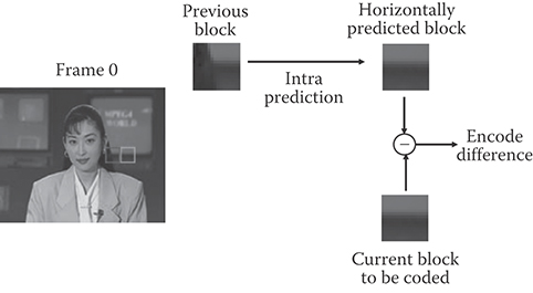
FIGURE 29.2 Example of spatial prediction.
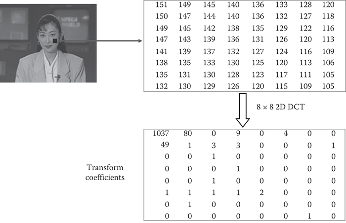
FIGURE 29.3 Spatial redundancy removal by 2D DCT.
29.1.2.2 Perceptual Redundancy Removal
Not all video data are equally significant from a perceptual point of view. For example, in the transform domain, the low-frequency components are perceptually more important than high-frequency components. By sending only the perceptually significant information, data compression can be achieved. Figure 29.4 shows an example where only 36 low frequency DCT coefficients (out of a total of 64 DCT coefficients) for each 8 × 8 block of data are retained. Also, the most significant bits (MSB) of transform coefficients are perceptually more important than the least significant bits (LSB). Quantization which reduces the number of bits used to represent a value also helps in perceptual redundancy removal since it leads to discarding of LSB information.

FIGURE 29.4 Perceptual redundancy removal. (a) Original frame and (b) image obtained by retaining 36 low frequency DCT coefficients for each 8 × 8 block.
29.1.2.3 Statistical Redundancy Removal
Not all video data in an image occurs with equal probability. Entropy coding can be used to reduce this statistical redundancy. For example, by using variable length coding (VLC), one can use shorter code words to represent frequent values and longer code words to present less frequent values. On the average this will require less number of bits to code video data than using fixed length coding to code the values. Table 29.1 shows an example of VLC. Assume that there are four types of symbols that need to be transmitted—A, B, C, and D—with probability of occurrence shown in Table 29.1. If one were to use fixed length coding to transmit these symbols, 2 bits per symbol would be required. So to transmit a sequence of A, A, B, D, A, A, A, A, one would require 16 bits. If a variable length code as shown in Table 29.1 were to be used, the number of bits required for transmission would be 1 + 1 + 2 + 3 + 1 + 1 + 1 + 1 = 11 bits.
Figure 29.5a shows the effect of using entropy coding on an example image. The original image uses 8 bits/pixel. If the image were directly coded using variable length code consisting of 256 alphabets, only 7.14 bits will be required to represent a pixel. Alternatively, when VLC is applied on transformed and quantized image (Figure 29.5b), only 1.82 bits will be required to code a pixel.
29.1.2.4 Temporal Redundancy Removal
Significant amount of temporal redundancy exists in video sequences as can be seen from Figure 29.1a where most of the background remains static from one image to the next. There are several ways in which temporal redundancy can be exploited to reduce data rate.
29.1.2.4.1 Conditional Replenishment
This technique encodes only the blocks that have changed from previous picture as shown in Figure 29.6a. The advantage of conditional replenishment is that it requires no additional frame buffers. The received blocks can be directly written into the display frame buffer.
29.1.2.4.2 Frame Difference Coding
This technique encodes frame differences as shown in Figure 29.6b. Difference blocks typically consume fewer bits than original blocks leading to frame difference coding providing better compression performance than conditional replenishment. However, unlike conditional replenishment, frame difference coding requires a previous frame buffer to be stored in decoder to reconstruct current frame.
TABLE 29.1 Example of Variable Length Coding
Symbol |
Probability of Occurrence |
Fixed Length Coding |
Variable Length Coding |
A |
0.5 |
00 |
0 |
B |
0.25 |
01 |
10 |
C |
0.125 |
10 |
110 |
D |
0.125 |
11 |
111 |
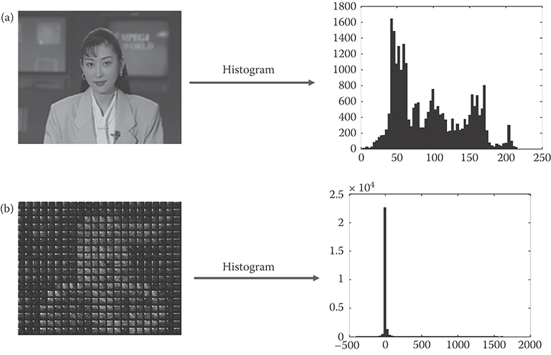
FIGURE 29.5 Effects of statistical redundancy removal on (a) original image: 8 bpp, entropy coding of original image: 7.14 bpp and (b) transformed and quantized image: 1.82 bpp.
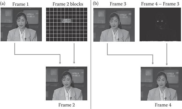
FIGURE 29.6 Temporal redundancy removal by (a) conditional replenishment and (b) frame difference coding.
29.1.2.4.3 Motion-Compensated Prediction (MCP)
Frame difference coding works well when there is no significant motion between pictures. When there is motion as shown in example of Figure 29.7, frame difference coding will lead to large differences. The motion between the frames needs to be compensated for before differencing. A popular way of doing this is to use block motion estimation (ME)/compensation. The frame is divided into blocks and, for each block in current picture, the relative motion between the current block and a matching block of the same size in the previous frame is determined through ME. A motion vector (mvx, mvy) is transmitted for each block to indicate the relative motion.
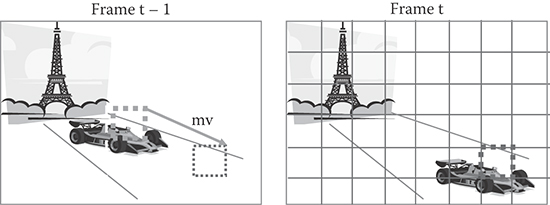
FIGURE 29.7 Example of MCP.
29.1.3 Basic Video Coding Architecture
A common approach in video coding is to combine motion estimation/compensation, spatial prediction, transform, quantization, and entropy coding into a hybrid scheme to exploit all forms of redundancies in video sequences. A video coding architecture that forms a basis of most of the existing video coding standards is shown in Figure 29.8.
Pictures are coded in either of the two modes—INTER or INTRA. In INTRA-coding, the current picture is encoded without any relation to the previous picture. Spatial prediction can be used to predict blocks of pixels from neighboring pixel values. In INTER coding, the current image is predicted from neighboring pictures using block motion compensation and the difference between the current image and the predicted image is encoded. Note that INTER coding requires that a copy of the neighboring pictures be stored in the frame buffer. The first picture in the video sequence is coded in the INTRA-mode to initialize the frame buffer. There are two types of INTER pictures—P picture and B picture as shown in Figure 29.9. P pictures are coded with respect past pictures where as B pictures are coded with respect to both past and future pictures.

FIGURE 29.8 Basic video coding architecture.
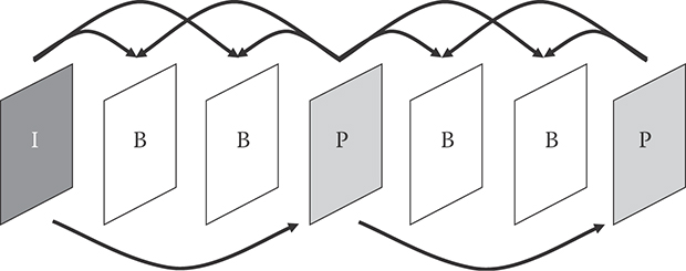
FIGURE 29.9 P and B pictures in IBBP GOP structure.
The basic unit of data operated on is called a macroblock (MB) and are the data (both luma and chroma components) corresponding to a block of 16 × 16 pixels. The input image is split into disjoint MBs and the processing is done on an MB basis. In INTER MBs, ME is performed on the MB to be encoded and motion vector (MV) is estimated between the current picture and neighboring picture for the MB to be encoded. ME is typically done using only the luma component of the video images. For chroma components, the luma MV is appropriately scaled to take care of the different spatial resolutions of the luma and chroma components before it is used. The motion compensation prediction error is calculated by subtracting each pixel in the MB with its motion-shifted counterpart in the neighboring picture. In INTRA-MBs, when spatial prediction is used, the prediction error is calculated by subtracting each pixel in MB from its spatial prediction from neighboring pixel values.
2D DCT is applied on prediction error (if spatial prediction or ME is used) or on original MB (if no prediction is used). The resulting DCT coefficients are then quantized. Depending on the quantization step size, this will result in a significant number of zero-valued coefficients. To efficiently encode the DCT coefficients which remain nonzero after quantization, the DCT coefficients are typically zig-zag scanned and run-length encoded. The run-length-encoded DCT coefficients and the MVs are variable length encoded before transmission. Arithmetic coding can also be used instead of VLC.
The decoder uses a reverse process to reproduce the MB at the receiver. After entropy decoding the received video bitstream, the pixel values of the prediction error are reconstructed by inverse quantization and inverse DCT. The spatially predicted pixels or the motion-compensated pixels from the neighboring picture contained in the frame buffer are added to the prediction error to reconstruct the particular MB transmitted. All MBs of a given picture are decoded and the whole picture is reconstructed.
29.1.4 Early Video Coding Standards
29.1.4.1 H.261
H.261 was standardized by ITU for videoconferencing over ISDN. H.261 supports two standard picture formats—the Common Intermediate Format (CIF–352 × 288) or the Quarter-CIF (QCIF, 176 × 144). The luma and chroma resolutions of the CIF and QCIF formats are summarized in Table 29.2. Pictures in H.261 are coded either in INTRA-mode or in INTER modes. Only P pictures are supported and a single MV at integer-pixel resolution is used for each MB. The MBs of either the image or the residual image are split into blocks of size 8 × 8 which are then transformed using DCT. The resulting DCT coefficient levels are quantized and run-length coded. The run-level pairs are variable length encoded. H.261 is typically operated at a bit rate of p × 64 kbps, where p is an integer from 1 to 30 [1].
TABLE 29.2 QCIF and CIF Resolutions
|
Luma |
Chroma |
QCIF |
176 × 144 |
88 × 72 |
CIF |
352 × 288 |
176 × 144 |
29.1.4.2 MPEG-1
MPEG-1 video standard was developed by ISO/IEC. It was designed to provide a digital equivalent of the popular VHS video tape. It is used in Video CD (VCD) with data rates of around 1.5 Mbps. Its supports YUV 4:2:0 video of SIF format (352 × 240 at 30 fps or 352 × 288 at 25 fps). Compared to H.261, MPEG-1 uses MVs at half-pixel resolution and supports both P and B pictures. It also introduced adaptive perceptual quantization where the step size used during quantization of various DCT coefficients can be adapted based on human visual perception considerations [2].
29.1.4.3 MPEG-2
MPEG-2 was developed for digital TV applications. It was built on top of MPEG-1 and introduced support for interlaced video which is used in TVs. MPEG-2 has become a very widely used standard and is used in DVDs, cable and satellite television, HDTVs, and Blu-ray discs. It supports higher resolution than MPEG-1, for example, standard definition TV (SDTV) resolution of 720 × 480 for NTSC and 720 × 576 for PAL, 1080i resolution of 1920 × 1080 interlaced etc. MPEG-2 is used at around 4–8 Mbps for SDTV applications and 10–20 Mbps for HDTV applications. Interlaced video coding tools introduced in MPEG-2 include: field pictures, field/frame motion compensation, MVs for 16 × 8 blocks, frame/field DCT. MPEG-2 also introduced tools for scalable video coding but these are not widely used [3].
29.1.4.4 H.263
H.263 was developed for videoconferencing over plain old telephone system (POTS) at data rates of 28.8 kbps. The video resolution targeted was sub-QCIF (128 × 96) and QCIF. Video conferencing at 28.8 Kbps ended up being very difficult and H.263 started getting used for video conferencing over ISDN and Internet since it provides better quality than H.261. Most of the improvements in H.263 come from using MVs with half-pixel resolution and from using improved VLC to encode DCT coefficients. DCT coefficients are coded using a 3D variable length code table that jointly codes DCT level, runs of zeros, and signaling of the last coefficient in the block. The core of H.263 specification is called the baseline profile. Several other optional modes were introduced in subsequent versions of H.263. These end up being called H.263+ and H.263++. Several of these options get used in the subsequent MPEG-4 simple profile and AVC/H.264 standard. Some of the options are [4]:
Unrestricted MV mode: In this mode, MVs are allowed to point to pixels outside the picture. The values used for the nonexistent “outside” pixels are simply the values of the corresponding pixels on the nearest edge of the picture. This mode is found to improve the picture quality when there is significant motion at the edges of the image.
MVs for 8 × 8 blocks.
Syntax-based arithmetic coding.
Multiple reference frames for motion compensation.
29.1.4.5 MPEG-4
MPEG-4 was designed to be a broad standard to cover various traditional and emerging applications areas: TV, film, wireless communications, 3D models, and so on. It has several parts: object-based coding, synthetic video coding, wavelet-based still texture coding, and natural video coding. Of all these, only the parts that cover coding of traditional video get used mainly in digital cameras, camcorder, and streaming video. The parts that get used are: MPEG-4 simple profile tools and advanced simple profile tools [5].
MPEG-4 Simple Profile is a superset of H.263 baseline profile. Additional tools include:
DCT coefficient prediction from neighboring block for intra coded MBs.
Unrestricted MV mode and MVs for 8 × 8 blocks.
Tools for improving error resilience of bitstreams.
Resync markers: Resync markers help in resynchronization of the bitstream in case of bitstream errors. Video data between resync markers is called a video packet and contains enough information to carry out decoding independent of neighboring video packet information. Because of the use of variable length encoding, bitstream errors can cause a loss of synchronization in entropy decoding and thereby lead to incorrect reconstruction of video pictures. Resync markers are unique and do not occur in the bitstream other than in the video packet header so a decoder that encounters bitstream errors can search for the next resync marker to achieve synchronization.
Data partitioning: In data partitioning, video data are split into two partitions with their own headers. The first partition consists of perceptually more significant information such as mode information and MVs. The second partition consists of coefficient data. In case the second partition is lost, the information in the first partition can be used to perform error concealment. Also channel coding techniques such as unequal error protection (UEP) can be used with data partitioning. UEP protects the more significant information at a higher level than the less significant information. So using UEP techniques, the first partition can be error protected more than the second partition.
Reversible VLC: These can be decoded in both the forward direction and the reverse direction. In the case of bitstream errors one could go to the end of the video packet and start decoding in reverse direction to try to salvage more information from the bitstream.
MPEG-4 advanced simple profile includes support for B pictures and interlaced tools. It also introduces MVs at quarter-pixel resolution and global motion compensation, which allows for signaling of motion parameters for the whole frame.
29.2 H.264/AVC
H.264/AVC (MPEG-4 Part 10) is the video coding standard developed by the joint efforts from ITU-T VCEG and ISO/IEC MPEG [6,7]. There was a call for proposal for H.26L in 1998, on which the start of H.264/AVC was based, and the joint video team (JVT) was formed in 2001 to start the standardization work jointly between VCEG and MPEG. Since the issuance of final draft international standard (FDIS) in 2003, H.264/AVC has been the state-of-the-art video coding standard that has been successfully deployed in various fields of industry including HDTV broadcasting, mobile and internet video services, digital cameras and camcorders, security systems, video conferencing systems, Blu-ray Disc, and so on [8].
Design of H.264/AVC codec inherits that of the previous standards such as MPEG-2 and H.263++. It uses block-based processing with motion prediction and transform coding. However, each traditional coding tool is optimized and new coding tools are introduced to achieve coding efficiency improvement. It has been reported that H.264/AVC can reduce bit rate by half at the same quality compared to its previous international standards [9].
The overview of H.264/AVC coding algorithm is given in Section 29.2.1. Section 29.2.2 discusses how optimal performance can be achieved at the encoder side in terms of coding efficiency. Usage of supplemental enhancement information (SEI) is also described. Finally, in Section 29.2.3, profile and level information is given along with visual quality analysis.
29.2.1 Coding Tools in H.264/AVC
The structure of H.264/AVC codec is similar to one shown in Figure 29.8. However, every coding block in H.264/AVC is improved by adopting new coding tools. This subsection highlights some of those tools.
29.2.1.1 High-Level Syntax and Data Structure
High-level syntax defines bitstream format and network abstraction layer (NAL) unit types. NAL unit types defined in H.264/AVC are shown in Table 29.3. Sequence parameter set (SPS) and picture parameter set (PPS) NAL units contain common information needed at the sequence level and picture level, respectively. SEI NAL unit is an optional NAL unit and can be included to provide additional information that will be useful for decoding or display processing. Coded slice NAL unit contains compressed video information. As shown in Figure 29.10, these form access units (i.e., decoded picture) and each access unit consists of single or multiple slices.
29.2.1.2 Intra Prediction
One of important tools introduced in H.264/AVC is the intra and inter prediction at MB level in variable block size partitions. The partitioned block sizes available for intra and inter predictions are different. When an MB is intra-coded, the MB is divided into the block sizes from 4 × 4 to 16 × 16 and the original pixels in each block are predicted from the reconstructed pixels in neighboring blocks to remove spatial correlation. Available prediction modes depend on color component and block size. For 4 × 4 and 8 × 8 luma block, 9 modes (1 DC + 8 directional) are defined as illustrated in Figure 29.11. For 16 × 16 luma, only 4 modes (1 DC + 3 directional) are defined. For chroma sample, only 8 × 8 intra prediction with the same modes as 16 × 16 luma prediction is allowed. However, the mode indices used for signaling 16 × 16 luma and 8 × 8 chroma prediction directions are slightly different as shown in Tables 29.4 and 29.5.
29.2.1.3 Inter Prediction (MCP)
An MB has more flexibility in its partition size when it is inter-coded. Figure 29.12 shows the partitions available for inter-coded MBs. The luma component can be partitioned into the smaller blocks of 16 × 16, 16 × 8, 8 × 16, or 8 × 8, and each 8 × 8 partition (i.e., sub-MB) can be partitioned again into the blocks of 8 × 8, 8 × 4, 4 × 8, or 4 × 4. The chroma component follows the luma partition after scaling according to the chroma format. Every partition in an inter-coded MB is predicted using its own reference picture and MV to remove temporal correlation as much as possible.
Table 29.3 H.264/AVC NAL Units (Nonshaded Rows) and Additional NAL Units for H.264/SVC (Shaded Rows)
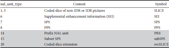

FIGURE 29.10 H.264/AVC NAL units and syntax structure.

FIGURE 29.11 Intra prediction modes for luma 4 × 4 and 8 × 8 blocks.
TABLE 29.4 Available Intra 16 × 16 Prediction Modes
Intra 16 × 16 PredMode |
Name of Intra 16 × 16 PredMode |
0 |
Intra_16 × 16_Vertical |
1 |
Intra_16 × 16_Horizontal |
2 |
Intra_16 × 16_DC |
3 |
Intra_16 × 16_Plane |
TABLE 29.5 Available IntraChroma Prediction Modes
Intrachroma_pred_mode |
Name of intra_chroma_pred_mode |
0 |
Intra_Chroma_DC |
1 |
Intra_Chroma_Horizontal |
2 |
Intra_Chroma_Vertical |
3 |
Intra_Chroma_Plane |

FIGURE 29.12 Available MB partitions and sub-MB partition for inter coded MB.
More than one previously coded picture can be employed for MCP in H.264/AVC. The maximum number of reference pictures that one picture can use is 16. However, since all the blocks in an 8 × 8 partition have the same reference picture, it is possible for one MB to have up to 4 reference pictures. To realize MCP with multiple reference pictures, the decoded picture buffer (DPB) is introduced, in which previously decoded pictures are stored. DPB provides ways to store and remove decoded pictures flexibly at any time. For example, decoded pictures can stay for a long time in DPB so that they can be used as a reference for successive pictures. By doing so, an H.264/AVC encoder can exploit both short-term and long-term dependencies between pictures.
MCP is performed using MVs at quarter-pixel resolution in H.264/AVC. Temporal prediction samples at finer fractional positions improve the performance of MCP significantly. For luma, the prediction samples at half-pixel positions are derived by filtering integer samples in horizontal and vertical direction separately using a 1-D 6-tap filter. The prediction samples at quarter-pixel positions are obtained by averaging adjacent integer sample and half-pixel sample. Fractional prediction samples for chroma are derived using bilinear interpolation. Because chroma resolution is half of luma resolution in the 4:2:0 format, a MV at quarter-pixel position in luma points to one-eighth sample in chroma.
When there are brightness changes between two pictures, that is, current and reference pictures, the residual signal after MCP will still have high energy even though there is no motion between pictures. Weighted prediction is introduced to improve coding efficiency in such cases, for example, fade-in and fade-out. By the weighted prediction technique, the prediction signal is modulated using scaling factor and offset, which is signaled in the bitstream, so that the brightness change between two pictures can be compensated [10,11].
The spatial direct mode in B picture in addition to temporal direct mode, which is already supported in the previous coding standards, is another source of coding efficiency improvement. With spatial direct mode, the forward and backward MVs of an MB are inferred from those of adjacent blocks, which is more efficient than temporal direct mode in many cases. The improvement of coding efficiency in H.264/AVC is also achieved by allowing B picture to be used as a reference for other pictures [12]. This change results in the use of hierarchical group of picture (GOP) structure. By applying finer quantization (i.e., higher quality) to lower layers that are used as references for higher layer, the coding efficiency can be improved when compared to the conventional IBBP structure of Figure 29.9. Since in H.264/AVC bi-predicted picture can be further used as a reference picture, a different notation is used to indicate bi-prediction picture—small letter b is used to indicate a bi-prediction picture that is not a reference picture and capital letter B is used to indicate a bi-prediction picture that is a reference picture. The conventionally used notation of IBBP coding of Figure 29.9 becomes IbbP coding in the new notation. It is worth noting that, as will be presented in detail in the next section, temporal scalability is supported without any changes by the hierarchical GOP structure.
29.2.1.4 Transform Coding and Quantization
H.264/AVC defines 4 × 4 and 8 × 8 block transforms. Both transforms are approximation of 2-D DCT [13] and can be applied by the use of adaptive block size transform (ABT) [14]. Note that only the inverse transform is the normative part defined by the standard. These transforms are integer transforms by means of shifting and multiplication operations, and the quantization is combined with transforms to avoid division operation. Therefore, they have very low computational complexity. Hadamard transform is also adopted into H.264/AVC for DC components in intra 16 × 16 mode and chroma coding.
29.2.1.5 Context-Adaptive Entropy Coding
Two context-adaptive entropy coding methods are supported: context-adaptive variable length coding (CAVLC) and context-adaptive binary arithmetic coding (CABAC) [15]. CAVLC is applied only to the coding of transform coefficients while normal VLC is used for the coding of other syntax elements. CAVLC encodes transform coefficients using VLC tables that adapt based on the number of nonzero coefficients of neighboring blocks. CABAC is applied to the coding of all the MB-level syntax elements, including MB header and transform coefficients. CABAC is the combination of binary arithmetic coding technique with context modeling, which consists of three operations of binarization, context modeling, and binary arithmetic coding. A syntax element is first converted to binary symbols called bin string and each bin is arithmetic coded with an updated context model. The context modeling is the key to high coding efficiency of CABAC. Based on the statistics of previously coded syntax elements, the probability model of binary symbols is updated and used to encode them. CABAC improves coding efficiency by around 9–14% over CAVLC at the cost of increased complexity.
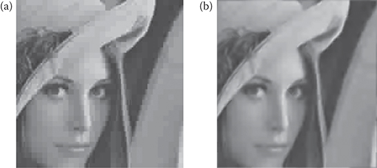
FIGURE 29.13 Visual quality comparison between decoded frames (a) without and (b) with deblocking filter.
29.2.1.6 In-Loop Deblocking Filter
Deblocking filter has been widely used as a postprocessing tool to remove blocking artifacts due to block-based processing used in video codecs. In H.264/AVC, deblocking filter is included inside the coding loop. A benefit of doing this is that coding efficiency improvement can be achieved by using the filtered reconstructed frame as reference frame. Both MB boundary and 4 × 4 block boundary are filtered with different filter strength according to properties such as prediction type, quantization parameter (QP) and so on. Figure 29.13 shows an example of output of H.264/AVC deblocking filter, which provides improved visual quality.
Various other coding tools are supported including interlaced coding, picture adaptive frame/field coding (PICAFF), MB adaptive frame/field coding (MBAFF), lossless coding, RGB coding, switching pictures, and so on.
29.2.2 Encoder Optimization and SEI
The H.264/AVC standard defines only the decoding process as normative part. However, it also provides a guideline and reference software for the encoder [16], which describes optimized mode selection scheme, adaptive rounding control, and so on. In addition, SEI can be used to improve the performance, especially for error resilience coding.
H.264/AVC provides various coding modes. For example, each MB can have intra or inter prediction type. Each prediction type consists of several modes as described in Section 29.2.1. Therefore, it is important to choose the optimal coding mode to improve coding efficiency, that is, to achieve less distortion at lower bitrate. The optimal solution can be found by using the Lagrangian optimization [17,18]. In general, an H.264/AVC encoder tries to calculate the actual bitrate and distortion incurred by each prediction mode, and calculates the rate-distortion (RD) cost as
where L and λ are Lagrange cost and Lagrange multiplier, respectively, D denotes sum of squared error (SSE), and R represents bitrate. The optimal Lagrange multiplier can be selected by taking derivative of distortion and bitrate of the compressed video as a function of quantization step size [19,20]. By exactly measuring bitrate and distortion for each prediction mode, the optimal coding mode can be selected.
Adaptive rounding control [21] is another encoding tool that improves coding efficiency by selecting a rounding offset value during the quantization process. The rounding offset value can be selected to adjust a deadzone size, and the adaptive rounding control accumulates statistics to find optimal offset value. This provides additional compression when the operating bitrate is very high. Various fast ME and fast mode decision algorithms are supported as well in the reference software.
SEI can also be used to improve the performance of H.264/AVC in different environments. SEI is a nonnormative part, which means that it is not mandatory for a decoder to support. However, an encoder can transmit information in the SEI, so that a decoder can support additional features. For example, spare picture SEI defines alternative reference frame to increase error resilience. Subsequence SEI enables UEP by defining hierarchical picture structure. Film grain SEI provides information to emulate film grain noise in an input sequence, so that similar noise can be reproduced at the decoder after coding the sequence without noise.
29.2.3 Profile Information and Performance Analysis
Profiles are defined to specify sets of coding tools used in different applications. A decoder can then conform to a particular profile without supporting all tools in H.264/AVC. In the first version of the standard, three profiles were defined; baseline, main, and extended profiles. Figure 29.14 shows the tools included in these profiles. Baseline profile includes less complex tools, for applications with limited resources, such as mobile applications.
Later, Fidelity Range Extension work [22,23] was added, which results in High, High 10, High 4:2:2, High 4:4:4 profiles. High profile, which includes ABT and quantization matrix in addition to the tools in main profile, is provided for the applications with less restriction in computation, memory, and power, such as HD broadcasting and storage like Blu-ray Disc. The other profiles are for applications requiring very high quality by supporting, for example, 10 bit per pixel, 4:2:2 and 4:4:4 or RGB color formats, lossless coding.
Similarly, levels are also specified for different application by defining maximum bitrate, buffer size, frame size, memory bandwidth, maximum MV range, and so on. For example, level 1 can only support resolutions up to 128 × 96 at 30.9 fps with 8 stored reference frames, and level 5.1 can support up to 4096 × 2048 at 30 fps with 5 stored reference frames.
Various studies have also been conducted to assess the performance of H.264/AVC compared to previous standards such as MPEG-2 and MPEG-4 in terms of bitrate reduction and visual quality. The verification test performed inside MPEG [9] reveals that H.264/AVC can achieve more than 50% of bitrate savings with better subjective quality. Figure 29.15 shows an example, where the Crew sequence is compressed using MPEG-2 at 10 Mbps, and H.264/AVC at 6 Mbps. H.264/AVC provides significantly better subjective quality compared to MPEG-2 with reduced blocking artifact and preservation of details in the scene. Another evaluation of H.264/AVC visual quality is also available in [24].

FIGURE 29.14 H.264/AVC profiles and coding tools.

FIGURE 29.15 Visual quality comparisons between coded frames by MPEG-2 and H.264/AVC encoders. (a) is a coded frame using MPEG-2 at 10 Mbps and (b) is a coded frame using H.264/AVC at 6 Mbps.
29.3 Scalable Video Coding
Scalable video coding is regarded as an attractive technique because of its potential advantages in providing a variety of transmission solutions over heterogeneous network environment to end-users with different sizes of display devices. By encoding an input video with scalable video coding techniques, a single scalable bitstream can be partially decoded at different levels of temporal and spatial resolution and fidelity depending on transmission channel bandwidth, display size, end-users’ preference, and so on. For this reason, scalable coding has drawn attentions in the applications such as personal media display, video streaming, and surveillance.
Simulcast is an alternative approach to scalable video. Multiple streams at various bitrates and resolutions are generated to accommodate different bandwidths and display sizes, and end-users select one of them depending on their conditions. However, this approach is inefficient in several aspects including poor coding efficiency. The size of multiple streams required to satisfy various network conditions may be large. Furthermore, it may not provide enough flexibility to switch among streams adaptively based on end-users’ conditions. Once one stream is selected, switching to others on the fly might be restricted or there could be significant drift errors due to switching.
The standardization effort for scalable video began from ISO/IEC MPEG-2 [3] and continued in MPEG-4 [5]. Scalable video coding has not been deployed successfully on a large scale in practical video coding systems mainly due to insufficient coding gain, flexibility and complexity issues. However, with availability of more powerful computing devices and improved coding efficiency by new coding techniques introduced in H.264/AVC [6], there has been an emerging interest again in scalable video coding. Recently, H.264/SVC has been standardized as a scalable extension of H.264/AVC. H.264/SVC aims to offer efficient scalable video coding at low complexity when compared with single-layer coding and simulcast while providing flexible formats of temporal, spatial, and SNR scalability. In this section, H.264/SVC is covered in detail with focus on its features and techniques adopted.
29.3.1 H.264/SVC Overview
H.264/SVC inherits all the features of H.264/AVC, which enable the production of a highly efficient video bitstream. Moreover, it is equipped with added features that support scalability by taking advantage of lower-layer signals in the higher layer encoding to minimize the redundant signal included in a compressed stream. There are mainly three types of scalability supported in the H.264/SVC standard: Temporal, spatial, and SNR scalability. In addition, they can be combined flexibly to provide multiple forms of scalability in a single stream. The coding efficiency of each scalable coding can be found in [25] and [26].
29.3.1.1 Temporal Scalability
Temporal scalability enables decoders to decode and display coded streams at variable frame rates without any drift error. It can be achieved by conventional IbbP GOP structure shown in Figure 29.16, where b picture is not used as a reference for other pictures. In this case, a decoder can display at reduced frame rates by decoding only I, or I and P pictures. In H.264/SVC, the temporal scalability is usually implemented by hierarchical GOP structure, in which pictures cannot use higher temporal-layer pictures as reference MC. Depending on the delay constraint, a GOP can be structured with hierarchical B or P pictures as shown in Figure 29.17, where the pictures at the lowest temporal layer, that is, T = 0, are called key pictures. It should be noted that the picture at temporal layer T = k use only reference picture whose T is smaller than or equal to k. Hierarchical B structure is realized by generalized B picture [12] that is used as reference as well for other pictures. While hierarchical B structure introduces a coding delay equal to the distance between two key pictures, there is no coding delay with hierarchical P structure. Suppose that the maximum frame rate is 60 fps when all pictures are decoded and displayed. With the GOP structures shown in Figure 29.17, a decoder can display at four different frame rates, for example, 7.5, 15, 30, and 60 fps by decoding T = 0, T = 0, 1, T = 0, 1, 2, and T = 0, 1, 2, 3, respectively. As stated in Section 29.2, the hierarchical GOP structure also improves coding efficiency, and temporal scalability can be realized as well in a H.264/AVC single-layer stream.
29.3.1.2 Spatial Scalability
The spatial scalability of H.264/SVC is based on the conventional layered coding approach with several inter-layer prediction techniques. Figure 29.18 demonstrates a two-layered spatial scalable video encoding process. Each picture of original input video in higher resolution is spatially decimated into a smaller resolution. Then the decimated picture is encoded by a base-layer (BL) encoder, which produces a bitstream fully compatible with the H.264/AVC standard. The original picture is encoded by an enhancement-layer (EL) encoder. The spatial scalable layer is identified by a dependency ID, D. Each EL picture can exploit the coded information of the previously coded BL picture at the same time instant by means of the following inter-layer prediction techniques. Note that the layer employed for inter-layer predictions is called a reference layer of the layer that exploits inter-layer predictions.
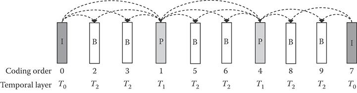
FIGURE 29.16 Temporal scalable coding by the conventional IbbP coding structure. Numbers and arrows represent the coding order and reference frames, respectively.

FIGURE 29.17 Temporal scalable coding by (a) hierarchical B picture and (b) hierarchical P pictures.

FIGURE 29.18 Two-layer spatial scalable video encoding process. (Adapted from H. Schwarz, D. Marpe, and T. Wiegand, IEEE Trans. Circuits and Syst. Video Technol., 17(9), 2007.)
29.3.1.2.1 Inter-Layer Intra Prediction
This method is used for intra-MB coding. When collocated blocks in a reference layer are intra coded, the reconstructed samples of collocated blocks can be up-sampled and used as the prediction signal for intra coding of the corresponding EL MB. This technique reduces bits of EL intra picture significantly.
29.3.1.2.2 Inter-Layer Motion Prediction
In the AVC base layer, MVs are predicted from neighboring blocks’ MVs (e.g., median of neighboring MVs) and their differences are coded. In H.264/SVC, when collocated blocks in a reference layer are inter coded, the corresponding EL MB can reuse their reference indices and scaled MVs for inter coding to reduce bits required to signal them.
29.3.1.2.3 Inter-Layer Residual Prediction
Residual signal still accounts for a significant portion of the bits at high bit rates and reference-layer residual signal can be utilized effectively to reduce bits to encode EL residual signal. The inter-layer residual prediction makes use of the up-sampled inverse-transformed residual signal as the prediction signal for the corresponding EL MB and encodes only the difference signal. The inter-layer residual prediction is employed only for EL inter MB coding when the collocated blocks in a reference layer are also inter coded.
29.3.1.2.4 Base Mode
Base mode is introduced to fully reuse MB mode information, MB partitions, MVs, and intra-information from the collocated blocks in a reference layer. If the collocated blocks are inter coded, base mode results in EL inter MB and its partitions, as well as MVs including reference indices, to be inferred from those of the collocated blocks. It means that the inter-layer motion prediction is switched on automatically with base mode flag. Inter-layer residual prediction can be switched on or off independently of base mode flag. In general, the residual signals in reference and enhancement layers are highly correlated to each other when base mode is enabled since MVs point to the same area in both layers. As a result, base mode works effectively along with inter-layer residual prediction. If the collocated blocks are intra coded, the base mode MB becomes intra-MB, which is called I_BL mode, and its samples are coded through the inter-layer intra prediction. Base mode is also quite effective in reducing intra coded MB bits.
29.3.1.3 SNR Scalability
H.264/SVC defines two types of SNR scalability, coarse-grain SNR (CGS) and medium-grain SNR (MGS) scalability. Fine-grain scalable coding was initially proposed, but it was not included finally in the standard.
In general, the CGS scalability is achieved by using different QP values across layers. The CGS design follows the same layered coding approach with the spatial scalability and the CGS layer is also identified by a dependency ID, D. CGS scalability is regarded as a special type of spatial scalability that does not involve any spatial resolution change between BL and EL. To be more specific, the input picture does not need to be decimated and all the inter-layer predictions are used without up-sampling of reference layer's reconstructed samples and residual signal and up-scaling of reference-layer's MVs. The only difference with spatial scalability is that the residual prediction in SNR scalability (i.e., both CGS and MGS) is performed in the transform domain before inverse transform.
The MGS layer is distinguished from CGS layers by its quality ID, Q. Multiple MGS layers can be added on top of the spatial or CGS layers, in which MGS layers should have different Q values. MGS scalability provides more flexible and dynamic ways for quality scalable coding. First of all, it supports DCT coefficient partitioning as well as all the scalable coding methods in CGS. All DCT coefficients are allowed to be divided into up to 16 partitions and each partition is sent in different layers. Second, it provides an improved method to trade-off coding efficiency and drift error, which is caused when the MCP processes at encoder and decoder are not synchronized. Unlike spatial and CGS enhancement layers, bitstream switching between MGS layers is allowed at any picture. Under such a scenario, the trade-off between coding efficiency and drift error is an important design issue and several control concepts have been proposed [25].
29.3.1.4 Combined Scalability
In common applications of scalable video, it is expected that a scalable global bitstream will contain all types of scalability. The H.264/SVC standard is designed to support any combination of temporal, spatial, and SNR scalability [27]. Accordingly, an H.264/SVC bitstream can provide great adaptation to the display resolution, channel bandwidth, quality level, and frame rate in various applications. Figure 29.19 shows an example of combined scalability in the T-D-Q space (the values of D, Q, and T represent spatial, quality, and temporal resolution of a slice), where each block in the space specifies an extractable layer representation. The desired layer is extracted and decoded with DQ ID. In H.264/SVC streams, all pictures are identified by distinct DQ ID, which is computed as (D << 4 + Q), and all pictures also have reference-layer DQ ID when any inter-layer prediction method is employed. It should be noted again that T is not necessary to identify a layer, since the temporal scalability is achieved within a layer. In general, a decoder needs to decode only one target layer, which is specified by the target values of T, D, and Q. Target T, D, and Q determine not only the target layer but also all reference layers required to decode the target layer.

FIGURE 29.19 Combined scalability in T-D-Q space. (Adapted from H. Schwarz et al., In Proc. ICME, 2005.)
29.3.2 Other H.264/SVC Features
There are other improvements for EL encoding in H.264/SVC besides inter-layer prediction methods. Some of them are briefly covered in this subsection.
29.3.2.1 Inter-Layer Deblocking Filter
In H.264/SVC, the inter-layer deblocking filter is proposed to improve inter-layer intra prediction for spatial scalable coding in addition to the existing deblocking filter. The new filter is intended to remove blocking artifacts in intra-MBs that are used as references for inter-layer intra prediction in spatial EL.
29.3.2.2 Skipped Slice
It is allowed to skip a whole slice in EL, for which only the number of MBs in the slice is signaled. When a slice is skipped, base mode and inter-layer residual prediction are used for all MBs inside it.
29.3.2.3 Intra–Inter Prediction Combination
In spatial scalable coding with the scaling factor other than 2, when base mode is enabled for an EL MB, the collocated blocks in a reference layer can contain both intra- and interblocks. When this occurs, the area mapped to the inter blocks in a reference layer is inter coded while other area is intra coded with inter-layer intra prediction.
29.3.3 H.264/SVC Bitstream Structure
Table 29.3 shows the important NAL units in H.264/SVC with their NAL unit types. In addition to the NAL units (1, 5, 7, and 8) in H.264/AVC, the H.264/SVC standard defines new NAL units to distinguish EL and BL and provides necessary information for scalable video decoding. They include prefix NAL unit, subset SPS, and coded slice extension. The coded slice extension has all MB parameters and data in the EL slice and the subset SPS has sequence-level parameters specific to EL. The prefix NAL unit is appended to the coded slices of BL, so that the information necessary for scalable video decoding can be assigned even to BL slices. Figure 29.20 illustrates the structures of NAL units. The NAL units of H.264/AVC consist of 1-byte header, which signals the NAL unit type and NAL unit payload. However, the prefix NAL unit and the coded slice extension have 3-byte NAL unit header extension between NAL unit header and payload, in which D, Q, and T IDs of a slice are signaled. The values of D, Q, and T represent spatial, quality, and temporal resolution of a slice and make it easy for a decoder to detect and extract the target layer that the decoder wants to display. It should be noted that the coded slice extension includes the payload of prefix NAL unit inside its payload.

FIGURE 29.20 H.264/SVC NAL unit structures.
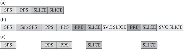
FIGURE 29.21 AVC bitstream extraction from SVC, (a) AVC bitstream, (b) SVC bitstream, and (c) extracted AVC bitstream from (b).
With the NAL units introduced in H.264/SVC, the generation of a SVC stream from multiple AVC streams and an AVC stream from one SVC stream can be completed simply by adding and removing new NAL units. For example, Figure 29.21 shows AVC, SVC, and extracted AVC stream formats. Suppose that a SVC stream is generated from two simulcast AVC streams. It can be done by adding the Prefix NAL units to coded slices of one AVC stream, converting SPS and coded slice of the other AVC stream to the subset SPS and coded slice extension, respectively and finally arranging them in the correct order. The AVC stream can be recovered again by identifying and removing SVC NAL units.
29.3.4 H.264/SVC Profiles
Three profiles are defined for H.264/SVC; Scalable Baseline, Scalable High, and Scalable High Intra profile. Scalable Baseline profile is defined on top of AVC Baseline profile. AVC base layers in the bitstreams conforming to this profile should be compliant to AVC baseline profile. For ELs, several coding tools allowed in AVC High profile, such as B picture, CABAC and 8 × 8 transform, are supported. However, interlaced, picture-adaptive field/frame (PICAFF) and MB adaptive field/frame (MBAFF) coding are not allowed. The biggest constraint for ELs is the scaling factor in spatial scalable coding. The scaling factor in SVC Baseline profile is limited to 2 and 1.5. However, there is no restriction to SNR and temporal scalable coding.
Scalable High profile is defined on top of AVC High profile. AVC base layers in the bitstreams conforming to this profile are compliant to AVC High profile. Most of the coding tools in AVC High profile are supported for ELs. Most importantly, arbitrary scaling factors other than 2 and 1.5 are supported for spatial scalable coding in SVC High profile. Scalable High Intra profile is defined for professional applications such as high-quality movies. The difference with Scalable High profile is that it uses only IDR coding for all layers.
29.4 Multiview Video Coding
The recent advances in camera and display technologies to capture and display multiple view signals, along with the desire for enhanced visual experiences, have brought about new video applications, namely, free viewpoint video (FVV) and stereo 3D video. FVV allows viewers to select any view point interactively, by which viewers can have sense of presence as if they are in the displayed scene. Stereo 3D video bring a new dimension of visual experience by showing left and right views to left and right eyes, respectively. The depth perceived in stereo 3D not only improves sense of presence but also makes the displayed scene look more natural. Stereo 3D video is now penetrating into daily life with the rapid development of consumer electronics such as TV, mobile phone, and tablet with stereo 3D support.
Due to huge raw bit rates of multiple views, the efficient coding of multiview video is key to the success of FVV and stereo 3D video. Accordingly, there have been several studies on compression techniques of multiview video. The simplest way is Simulcast that encodes all the views independently using any existing single-view encoder. However, this results in poor coding efficiency as expected. Recent standardization efforts for multiview video coding have extended the H.264/AVC standard. H.264/AVC has introduced stereo video information and frame packing arrangement SEI messages to support stereo 3D video. And the multiview extension of H.264/AVC, H.264/MVC, has been standardized for highly efficient multiview coding. There is also another activity toward a new 3D video standard under the ISO/IEC MPEG organization. This section introduces these multiview and 3D video coding techniques.
29.4.1 H.264/MVC Overview
H.264/MVC, which is extended from the H.264/AVC standards, has been designed to support efficient coding of multiple views into a single bitstream. Figure 29.22 shows the overall structure of a H.264/MVC system. The temporally synchronized videos from multiple cameras are fed into the H.264/MVC encoder to be coded into a single bitstream. Based on the fact that spatially neighboring pictures are correlated, the encoder saves bits required to encode additional views using so-called interview prediction. The coded stream is decoded and displayed by the H.264/MVC decoder in several ways depending on application. For FVV applications, the decoder decodes the desired view only, that is, target view, among multiple views and can switch the target view whenever necessary. For 3D video application, it is also possible to decode stereo views.
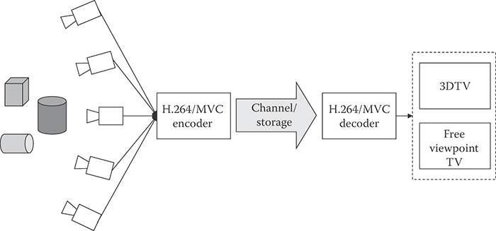
FIGURE 29.22 Multiview video system using H.264/MVC encoder/decoder.
Multiple camera sources can be encoded using various prediction structures, which might depend on camera array size and structures, for example, parallel or circular. Figure 29.23 depicts an exemplary prediction structure in the case of stereo-view encoding, where left view is an AVC base view that is always encoded independently. Figure 29.23a is the simplest way that encodes all views independently without interview prediction. However, as shown in Figure 29.23b and (c), the coding efficiency is improved by allowing nonbase views to be predicted from neighboring views for anchor (I or P) pictures, or both anchor and nonanchor pictures (B), respectively. In general, the interview prediction is more effective for anchor pictures than for nonanchor picture. The performance of interview prediction is well studied in [28].
The same NAL units in Table 29.3 are used for H.264/MVC as well, although their contents are quite different from those for H.264/SVC. For example, the prefix NAL unit and coded slice extension stream have NAL unit header extension between NAL unit header and payload. However, the NAL unit header extension in MVC has different syntax elements such as view ID and interview flag as shown in Figure 29.24. The coded slice extension in MVC is the same to the coded slice (nal_unit_type = 1 or 5) except for the reference picture list generation process due to interview prediction. It means that there is no MB-level change like inter-layer prediction in SVC for enhancement view encoding. The interview prediction is simply realized by adding reconstructed neighboring view pictures in the reference list of the current view. Therefore, the H.264/AVC encoder can be easily extended to support multiview coding.
There are two profiles defined for in H.264/MVC, namely, Multiview High profile and Stereo High profile. The main difference between two profiles is the number of views in a stream. Multiview High profile, which allows more than two views, is defined on top of the AVC High profile with some restrictions. For example, the interlaced picture coding tools including PICAFF and MBAFF are not supported in this profile. The AVC base view in the Stereo High profile is compliant to the AVC High profile as well.
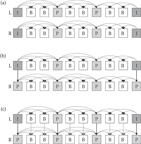
FIGURE 29.23 Prediction structure in H.264/MVC encoder for stereo-view coding, (a) simulcast, (b) interview prediction for anchor frames, and (c) interview prediction for all frames.
![]()
FIGURE 29.24 MVC NAL Unit header extension format.
However, the interlaced picture coding tools can be supported in the Stereo High profile, which allows only up to two views.
29.4.2 Stereo 3D Video Coding via H.264/AVC SEI Messages
There are two H.264/AVC SEI messages for stereo 3D video, stereo video information SEI and frame packing arrangement SEI. They are used to support stereo 3D video in H.264/AVC without any change of actual encoding and decoding process. Specifically, they inform a decoder how the decoded picture is generated from two pictures, and the decoder rearranges the decoded picture based on this information for display purpose.
Figure 29.25 describes the overall structure of a 3D video system of H.264/AVC with SEI messages. In the encoder side, temporally synchronized left and right view sequences go through the down converter, by which each picture of left and right view sequences is down-sized by 2 based on the SEI message. The down-sized left and right views are composed into a single picture and coded by an H.264/AVC encoder. In the decoder side, the decoded picture by an H.264/AVC decoder is decomposed into left and right views and both views are up-converted into the original size based on the SEI message. The stereo information and frame packing arrangement SEI messages are similar as both follow the structure in Figure 29.25; however, they define different down- and up-conversion formats. One of formats in the stereo information SEI message is illustrated in Figure 29.26, for which the interview prediction can be realized. As shown in Figure 29.27, by encoding each field separately and allowing bottom field to refer top field, we can have the same effect as the interview prediction in H.264/MVC, with the reduced resolution.
The disadvantage of 3D video by the SEI messages is that it reduces the resolutions of both views by half. However, it is very attractive because it is compatible to existing H.264/AVC codecs and infrastructures. Using the SEI messages, stereo 3D video can be brought to home via existing devices like DVD and Blu-ray players and 3D display with minimal efforts. There is also standardization activity to support full resolution stereo 3D video with the similar approach [29].
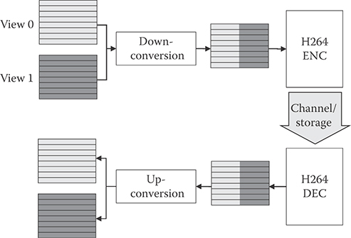
FIGURE 29.25 3D video system using H/264/AVC with side-by-side frame packing SEI messages.
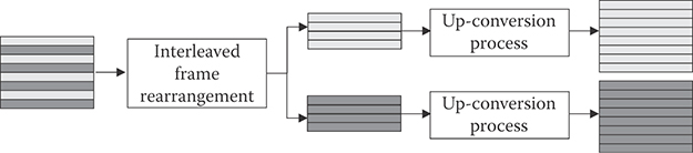
FIGURE 29.26 Rearrangement and up-conversion of interleaved picture using stereo information SEI message.

FIGURE 29.27 Stereo video coding of interleaved picture using stereo information SEI message.
29.4.3 MPEG 3D Video
Although the H.264/MVC standard reduces the redundancy by using interview prediction, the amount of data to be stored or transmitted is still very large especially when many views are captured and coded. Improvements to the interview prediction in H.264/MVC are currently being studied. For instance, the illumination and focus mismatch compensation method was proposed in [30], by which the different illumination conditions and focal lengths between a target view and a reference view are compensated for improved interview prediction. In [31] and [32], the interview prediction methods using view interpolation were proposed. In these methods, a target view is synthesized first based on neighboring views and this estimated target view is used as a reference for interview prediction while encoding the target view. The differential signal between the target view and the estimated target view is coded in a stream.
The idea of view interpolation is also applied to a new 3D video format of view plus depth [33]. Figure 29.28 illustrates the overall structure of a 3D system with a view-plus-depth format. The encoder encodes two views and depths into the view-plus-depth format. The decoder not only decodes coded views and depths but also synthesizes any intermediate view using depth image-based rendering (DIBR) technique [34]. Additional data could also be sent in a stream so that the decoder can have better quality of synthesized intermediate view. This 3D video representation is expected to be the most efficient way for multiview video application. However, there are several issues to be addressed for this system.
First, in the case that a ground-truth depth map is not available, the generation of high-quality depth map is the most fundamental issue. While there exist many depth map estimation methods in the literatures [35,36], these methods need to be evaluated in terms of synthesized views’ quality to develop the best depth map estimation method for this system. Regardless of whether depth map is ground truth or not, an efficient coding method for depth map should be developed. Since depth map has different characteristic from view picture, conventional video compression techniques may not be efficient. Exploiting the specific characteristics of depth map can enable higher coding efficiency. Second, it should be guaranteed that a view synthesis method employed always generates acceptable intermediate views. The quality of synthesized views will depend on the quality of coded views and depth maps, and the quality of coded and synthesized views should have similar quality. However, when there are large occluded areas between two coded views, it is not easy to synthesize intermediate views as good as coded views. To resolve this issue, the study on the additional data and its transmission method to improve synthesized views’ quality at minimum overhead is also essential [37].

FIGURE 29.28 3D video system with a view plus depth format.
The standardization effort for the 3D video coding with view-plus-depth format is being led by the ISO/IEC MPEG organization. They recently issued call for proposal [38] with common test sequences and environment. The primary goal is to define the data format and coding technology to enable high-quality reconstruction of coded and synthesized views for both stereoscopic 3D display and auto-stereoscopic multiview displays. All the issues mentioned in the above are expected to be addressed in the standard.
29.5 High-Efficiency Video Coding
High-efficiency video coding is the next-generation video coding standard currently being developed by the Joint Collaborative Team on Video Coding (JCT-VC) of ITU-T WP3/16 and ISO/IEC JTC 1/SC 29/WG 11 [39]. It is expected to provide around 50% improvement in coding efficiency compared with its predecessor H.264/AVC. The call for proposals occurred in January 2011 and the final draft international standard (FDIS) is expected to be completed in January 2013. In this section, the various new tools that have been adopted into the working draft (WD) of HEVC, based on the outcome of the sixth JCT-VC meeting held in July 2011, are discussed and the differences from H.264/AVC are highlighted.
29.5.1 Coding Block Structure
HEVC is intended for larger resolutions and higher frame rates. Accordingly, HEVC uses larger “macroblocks (MB)” compared to H.264/AVC. In HEVC, the largest coding unit (LCU) is 64 × 64 pixels, which is 16 times larger than the 16 × 16 pixel MB used in H.264/AVC. Using a large coding unit helps to improve coding efficiency, particularly for high resolutions where many pixels may share the same characteristics. The largest coding unit can be divided into smaller coding units (CU) using a quadtree structure as shown in Figure 29.29. A split flag is transmitted to indicate whether a CU should be divided into four smaller CUs. The smallest coding unit (SCU) allowed in HEVC is 8 × 8 pixels. An additional feature in HEVC is that within an LCU, there can be a mixture of inter and intra coding units. The CU can be further divided into prediction units (PU). The PU within a coding unit will undergo the same form of prediction (either all inter or all intra). The allowed PU sizes within a CU depend on whether the CU is inter- or intra predicted. Asymmetric motion partitions (AMP) are allowed for inter predicted PU.

FIGURE 29.29 Coding block structure in HEVC, (a) shows how an LCU is partitioned into CU with a quadtree structure and a mixture of inter predicted (gray) and intra predicted (white) CUs are allowed and (b) shows how CU are further divided into PUs.
29.5.2 Inter Prediction
Similar to H.264/AVC, quarter-pixel resolution MVs are supported in HEVC. HEVC uses a larger 8-tap DCT interpolation filter (DCTIF) that operates directly on the integer pixels rather than the two step 6-tap approach used in H.264/AVC. In addition, advanced motion vector prediction (AMVP) is used to signal the MV data. Compared to H.264/AVC, more neighbors are used for MV prediction. To signal skip or direct mode, merge mode is used, where multiple neighbors are used to predict the MVs and reference index.
29.5.3 Intra Prediction
Depending on the PU size, up to 34 directional modes are used for intra prediction of luma pixels. In addition, there are separate planar and DC modes. Depending on the prediction mode, intrasmoothing is applied to the reference pixels. For chroma pixels, four directional modes can be used, one of which can be the same as the luma mode. In addition, luma-based chroma prediction (LM chroma) can be used where chroma intra prediction is performed using the reconstructed luma pixels.
29.5.4 Transform
To support the larger resolutions, HEVC uses transforms from 4 × 4 up to 32 × 32. For a given coding unit, the transform sizes are signaled using a residual quadtree (RQT). For example, a CU of size 16 × 16 can be split into 16 4x4 transforms using a quadtree of depth 2.
For 4 × 4, based on intramode, a discrete sine transform (DST) is used for certain prediction modes. Nonsquare transforms (NSQT) with sizes 4 × 16/16 × 4, 8 × 32/32 × 8 are allowed for residual of inter prediction. An adaptive scan order is used for intrapredicted coefficients to map them from the 2-D transform to the 1-D set of coefficients to be coded by the entropy coder.
29.5.5 Loop Filters
A deblocking filter is applied to the 8 × 8 edges. Similar to H.264/AVC there is both a strong filter, which is applied to 3 pixels on either side of the edge, and a weak filter, which is applied to 2 pixels on either side of the edge. The chroma filter affects 1 pixel on either side of the edge.
Two additional loop filters shown in Figure 29.30 are used in HEVC: sample adaptive offset (SAO) and adaptive loop filter (ALF). After the deblocking filter, SAO is applied on a pixel basis based on the neighboring information. There are two methods of determining the offset with SAO: band offset and edge offset. In band offset, the size of the offset is determined based on the magnitude of the pixel. In edge offset, a two-point gradient is taken around the pixel and the difference dictates the offset that is to be added to the pixel. SAO can be enabled and disabled on an LCU basis, and is signaled using a quadtree.
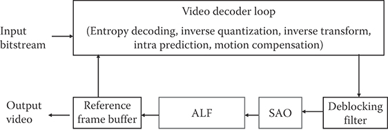
FIGURE 29.30 In-loop filters in HEVC. Adaptive loop filter (ALF) and sample adaptive offset (SAO) are two additional filters highlighted in red.
ALF is an adaptive FIR Wiener filter, which is applied after SAO. The number of filters taps in ALF can change for each slice; within each slice, there are sixteen sets of coefficients. There are two methods of selecting the coefficients: region-based and block-based. Region-based ALF involves breaking a frame into sixteen regions (i.e., dividing the frame into four in both vertical and horizontal directions). A coefficient set can be assigned to each region and all pixels within each region will use the same coefficient set. In block-based ALF, the coefficient set is selected based on the local characteristics of a given block of pixels. A separate filter is used for the chroma components. ALF can be enabled and disabled using the existing CU quadtree of the coding block structure.
29.5.6 Entropy Coding
Similar to H.264/AVC, HEVC uses context adaptive binary arithmetic coding (CABAC). However, improvements have been made to CABAC to enable higher throughput. This includes changes to the binarization and context selection of various syntax elements such as coefficient level, to reduce the number of context coded bins as well as overall number of bins. Bins are also reordered such that context coded bins with similar contexts are grouped together to enable parallel context processing, and bypass bins are grouped together to enable higher throughput.
References
1. Video codec for audiovisual services at p × 64 Kbits/s, ITU-T, Rec. H.261, ITU-T, March 1993.
2. Coding of moving pictures and associated audio for digital storage medic at up to about 1.5 Mbits/s, Part 2: Video, ISO/IEC 11172-2, March 1993.
3. Generic coding of moving pictures and associated audio information, Part 2: Video, ITU-T Rec. H.262 and ISO/IEC 13818-2, November 1994.
4. Video codec for low bit rate communication, ITU-T, Rec. H.263, ITU-T, January 1998.
5. Coding of audiovisual objects, Part 2: Visual, ISO/IEC 14496-2, ISO/IEC JTC 1, May 2004.
6. Advanced video coding for generic audiovisual services, ITU-T Rec. H.264 and ISO/IEC 14496-10, ITU-T and ISO/IEC JTC1, April 2007.
7. T. Wiegand, G. J. Sullivan, G. Bjøntegaard, and A. Luthra, Overview of the H.264/AVC video coding standard. IEEE Trans. Circuits Syst. Video Technol., 13(7), 560–576, 2003.
8. G. Sullivan, Overview of known H.264/MPEG-4 pt. 10/AVC deployment plans and status, Joint Video Team (JVT) of ISO/IEC MPEG & ITU-T VCEG, Document JVT-L009, Jul. 2004.
9. JVT and Test and Video Group, Report of the formal verification tests on AVC/H.264, ISO/IEC JTC1/SC29/WG11, Document N6231, Dec. 2003.
10. J. M. Boyce, Weighted prediction in the H.264/MPEG AVC video coding standard, in Proc. ISCAS, 2004.
11. D.-K. Kwon and H. J. Kim, Region-based weighted prediction for real-time H.264 encoder, in Proc. ICCE, 2011.
12. M. Flierl and B. Girod, Generalized B pictures and the draft H.264/AVC video compression standard. IEEE Trans. Circuits and Syst. Video Technol., 13(7), 2003.
13. H. Malvar, A. Hallapuro, M. Karczewicz, and L. Kerofsky, Low-complexity transform and quantization in H.264/AVC. IEEE Trans. Circuits Syst. Video Technol., 13(7), 598–603, 2003.
14. M. Wien, Variable block-size transforms for H.264/AVC, IEEE Trans. Circuits Syst. Video Technol. 13(7), 604–613, 2003.
15. D. Marpe, H. Schwarz, and T. Wiegand, Context-based adaptive binary arithmetic coding in the H.264/AVC video compression standard. IEEE Trans. Circuits and Syst. Video Technol., 13(7), 2003.
16. A. M. Tourapis, A. Leontaris, K. Sühring, and G. Sullivan, H.264/14496-10 AVC Reference Software Manual (revised for JM 17.1), Joint Video Team (JVT) of ISO/IEC MPEG & ITU-T VCEG, Document JVT-AE010, June 2009.
17. A. Ortega and K. Ramchandran. Rate-distortion techniques in image and video compression. IEEE Signal Proc. Magazine, 15(6), 23–50, 1998.
18. G. J. Sullivan and T. Wiegand. Rate-distortion optimization for video compression. IEEE Signal Proc. Magazine, 15(6), 74–90, 1998.
19. T. Wiegand and B. Girod. Lagrange multiplier selection in hybrid video coder control. In Proc. of IEEE Int. Conf. Image Proc., ICIP 2009, pp. 542–545, Cairo, Egypt, Oct. 2001.
20. T. Wiegand, H. Schwarz, A. Joch, F. Kossentini, and G. J. Sullivan. Rate constrained coder control and comparison of video coding standards. IEEE Trans. Circuits Syst. Video Technol., 13(7), 688–703, 2003.
21. G. Sullivan, Adaptive quantization encoding technique using an equal expected-value rule, Joint Video Team (JVT) of ISO/IEC MPEG & ITU-T VCEG, Document JVT-N011, Jan. 2005.
22. G. J. Sullivan, P. Topiwala, and A. Luthra, The H.264/AVC Advanced video coding standard: Overview and introduction to the Fidelity Range Extensions. SPIE Conference on Applications of Digital Image Processing XXVII, Aug., 2004.
23. D. Marpe, T. Wiegand, S. Gordon, H.264/MPEG4-AVC Fidelity Range Extensions: Tools, profiles, performance, and application areas. In Proc. of IEEE Int. Conf. Image Proc., ICIP 2005, Sep. 2005.
24. T. Oelbaum, V. Baroncini, T. K. Tan, and C. Fenimore, Subjective quality assessment of the emerging AVC/H.264 video coding standard. International Broadcasting Conference (IBC), Sep., 2004.
25. H. Schwarz, D. Marpe, and T. Wiegand, Overview of the scalable video coding extension of the H.264/AVC standard. IEEE Trans. Circuits and Syst. Video Technol., 17(9), 2007.
26. M. Wien, H. Schwarz, and T. Oelbaum, Performance analysis of SVC. IEEE Trans. Circuits and Syst. Video Technol., 17(9), 2007.
27. H. Schwarz, D. Marpe, T. Schierl, and T. Wiegand, Combined scalability support for the scalable extension of H.264/AVC. In Proc. ICME, 2005.
28. P. Merkle, A. Smolic, K. Muller, and T. Wiegand, Efficient prediction structure for multiview video coding. IEEE Trans. Circuits and Syst. Video Technol., 17(9), 2007.
29. A. M. Tourapis, P. Pahalawatta, A. Leontaris, Y. He, Y. Ye, K. Stec, and W. Husak, A frame compatible system for 3D delivery, ISO/IEC JCT1/SC29/WG11, Doc. M17925, July 2010.
30. J. H. Kim, P. Lai, and A. Ortega, New coding tools for illumination and focus mismatch compensation in multiview video coding. IEEE Trans. Circuits and Syst. Video Technol., 17(11), 2007.
31. K. Yamamoto, M. Kitahara, H. Kimata, T. Yendo, T. Fujii, M. Tanimoto, S. Shimizu, K. Kamikura, and Y. Yashima, Multiview video coding using view interpolation and color correction. IEEE Trans. Circuits and Syst. Video Technol., 17(11), 2007.
32. K. N. Iyer, K. Maiti, B. Navathe, H. Kannan, and A. Sharma, Multiview video coding using depth based 3D warping. In Proc. ICME, 2008.
33. P. Merkle, A. Smolic, K. Muller, and T. Wiegand, Multi-view video plus depth representation and coding. In Proc. ICIP, 2007.
34. C. Fehn, Depth-image-based rendering (DIBR), compression and transmission for a new approach on 3D-TV. In Proc. SPIE, 2004.
35. S. Ince, E. Martinian, S. Yea, and A. Vetro, Depth estimation for view synthesis in multiview video coding. In 3DTV conference, 2007.
36. Q. Zhang, P. An, Y. Zhang, L. Shen, and Z. Zhang, Improved multi-view depth estimation for view synthesis in 3D video coding. In 3DTV conference, 2011.
37. W. S. Kim, A. Ortega, J. Lee, and H. Wey, 3-D video coding using depth transition data. In Proc. Picture Coding Symposium, December 2010.
38. Call for Proposals on 3D video coding technology, ISO/IEC JCT1/SC29/WG11, Doc. N12036, March 2011.
39. B. Bross, W.-J. Han, J.-R. Ohm, G. J. Sullivan, T. Wiegand, WD4: Working Draft 4 of High-Efficiency Video Coding, JCTVC-F803, JCT-VC, 6th Meeting: Torino, IT, July14-22, 2011.