15 Optimum Receivers

Every engineer strives for optimality in design. This is particularly true for communications engineers since in many cases implementing sub optimal receivers and sources can result in dramatic losses in performance. As such, this chapter focuses on design principles leading to the implementation of optimum receivers for the most common communication environments.

The main objective in digital communications is to transmit a sequence of bits to a remote location with the highest degree of accuracy. This is accomplished by first representing bits (or more generally short bit sequences) by distinct waveforms of finite time duration. These time-limited waveforms are then transmitted (broadcasted) to the remote sites in accordance with the data sequence.

Unfortunately, because of the nature of the communication channel, the remote location receives a corrupted version of the concatenated signal waveforms. The most widely accepted model for the communication channel is the so-called additive white Gaussian noise^* channel (AWGN channel). Mathematical arguments based upon the central limit theorem [7], together with supporting empirical evidence, demonstrate that many common communication channels are accurately modeled by this abstraction. Moreover, from the design perspective, this is quite fortuitous since design and analysis with respect to this channel model is relatively straightforward.

*For those unfamiliar with AWGN, a random process (waveform) is formally said to be white Gaussian noise if all collections of instantaneous observations of the process are jointly Gaussian and mutually independent. An important consequence of this property is that the power spectral density of the process is a constant with respect to frequency variation (spectrally flat). For more on AWGN, see Papoulis [4].

15.2 Preliminaries

To better describe the digital communications process, we shall first elaborate on so-called binary communications. In this case, when the source wishes to transmit a bit value of 0, the transmitter broadcasts a specified waveform s₀(t) over the bit interval t ∈ [0, T]. Conversely, if the source seeks to transmit the bit value of 1, the transmitter alternatively broadcasts the signal s₁(t) over the same bit interval. The received waveform R(t) corresponding to the first bit is then appropriately described by the following hypotheses testing problem:

\begin{array}{l} H_{0} : R (t) = s_{0} (t) + η (t) 0 \leq t \leq T \\ H_{1} : R (t) = s_{1} (t) + η (t) \end{array} (15.1)

$\begin{array}{l} H_{0} : R (t) = s_{0} (t) + η (t) 0 \leq t \leq T \\ H_{1} : R (t) = s_{1} (t) + η (t) \end{array} (15.1)$

where, as stated previously, η(t) corresponds to AWGN with spectral height nominally given by N₀/2. It is the objective of the receiver to determine the bit value, that is, the most accurate hypothesis from the received waveform R(t).

The optimality criterion of choice in digital communication applications is the total probability of error normally denoted as P_e. This scalar quantity is expressed as

\begin{array}{l} P_{e} = P r (declaring 1|0 transmitted) P r (0 transmitted) \\ + P r (declaring 0|1 transmitted) P r (1 transmitted) \end{array} (15.2)

$\begin{array}{l} P_{e} = P r (declaring 1|0 transmitted) P r (0 transmitted) \\ + P r (declaring 0|1 transmitted) P r (1 transmitted) \end{array} (15.2)$

The problem of determining the optimal binary receiver with respect to the probability of error is solved by applying stochastic representation theory [10] to detection theory [5,9]. The specific waveform representation of relevance in this application is the Karhunen–Loève (KL) expansion.

15.3 Karhunen–Loève Expansion

The Karhunen–Loève expansion is a generalization of the Fourier series designed to represent a random process in terms of deterministic basis functions and uncorrelated random variables derived from the process. Whereas the Fourier series allows one to model or represent deterministic time-limited energy signals in terms of linear combinations of complex exponential waveforms, the Karhunen–Loève expansion allows us to represent a second-order random process in terms of a set of orthonormal basis functions scaled by a sequence of random variables. The objective in this representation is to choose the basis of time functions so that the coefficients in the expansion are mutually uncorrelated random variables.

To be more precise, if R(t) is a zero mean second-order random process defined over [0, T] with covariance function K_R(t, s), then so long as the basis of deterministic functions satisfy certain integral constraints [9], one may write R(t) as

R (t) = \sum_{i = 1}^{\infty} R_{i} ϕ_{i} (t) 0 \leq t \leq T (15.3)

$R (t) = \sum_{i = 1}^{\infty} R_{i} ϕ_{i} (t) 0 \leq t \leq T (15.3)$

where

R_{i} = \int_{0}^{T} R (t) ϕ_{i} (t) d t

$R_{i} = \int_{0}^{T} R (t) ϕ_{i} (t) d t$

In this case the R_i will be mutually uncorrelated random variables with the φ_i being deterministic basis functions that are complete in the space of square-integrable time functions over [0, T]. Importantly, in this case, equality is to be interpreted as mean-square equivalence, that is,

\lim_{N \to \infty} E [{(R (t) - \sum_{i = 1}^{N} R_{i} ϕ_{i} (t))}^{2}] = 0

$\lim_{N \to \infty} E [{(R (t) - \sum_{i = 1}^{N} R_{i} ϕ_{i} (t))}^{2}] = 0$

for all 0 ≤ t ≤ T.

FACT 15.1: If R(t) is AWGN, then any basis of the vector space of square-integrable signals over [0, T] results in uncorrelated and therefore independent Gaussian random variables.

The use of Fact 15.1 allows for a conversion of a continuous time detection problem into a finite-dimensional detection problem. Proceeding, to derive the optimal binary receiver, we first construct our set of basis functions as the set of functions defined over t ∈ [0, T] beginning with the signals of interest s₀(t) and s₁(t). That is,

{s_{0} (t), s_{1} (t), plus a countable number of functions which complete the basis} .

${s_{0} (t), s_{1} (t), plus a countable number of functions which complete the basis} .$

In order to ensure that the basis is orthonormal, we must apply the Gramm–Schmidt procedure^* [6] to the full set of functions beginning with s₀(t) and s₁(t) to arrive at our final choice of basis {φ_i(t)}.

FACT 15.2: Let {φ_i(t)} be the resultant set of basis functions.

Then for all i > 2, the φ_i(t) are orthogonal to s₀(t) and s₁(t). That is,

\int_{0}^{T} ϕ_{i} (t) s_{j} (t) d t = 0

$\int_{0}^{T} ϕ_{i} (t) s_{j} (t) d t = 0$

for all i > 2 and j = 0,1.

Using this fact in conjunction with Equation 15.3, one may recognize that only the coefficients R₁ and R₂ are functions of our signals of interest. Moreover, since the R_i are mutually independent, the optimal receiver will, therefore, only be a function of these two values.

Thus, through the application of the KL expansion, we arrive at an equivalent hypothesis testing problem to that given in Equation 15.1,

\begin{array}{l} H_{0} : R = [\begin{array}{l} \int_{0}^{T} ϕ_{1} (t) s_{0} (t) d t \\ \int_{0}^{T} ϕ_{2} (t) s_{0} (t) d t \end{array}] + [\begin{matrix} η_{1} \\ η_{2} \end{matrix}] \\ H_{1} : R = [\begin{array}{l} \int_{0}^{T} ϕ_{1} (t) s_{1} (t) d t \\ \int_{0}^{T} ϕ_{2} (t) s_{1} (t) d t \end{array}] + [\begin{matrix} η_{1} \\ η_{2} \end{matrix}] \end{array} (15.4)

$\begin{array}{l} H_{0} : R = [\begin{array}{l} \int_{0}^{T} ϕ_{1} (t) s_{0} (t) d t \\ \int_{0}^{T} ϕ_{2} (t) s_{0} (t) d t \end{array}] + [\begin{matrix} η_{1} \\ η_{2} \end{matrix}] \\ H_{1} : R = [\begin{array}{l} \int_{0}^{T} ϕ_{1} (t) s_{1} (t) d t \\ \int_{0}^{T} ϕ_{2} (t) s_{1} (t) d t \end{array}] + [\begin{matrix} η_{1} \\ η_{2} \end{matrix}] \end{array} (15.4)$

where it is easily shown that η₁ and η₂ are mutually independent, zero-mean, Gaussian random variables with variance given by N₀/2, and where φ₁ and φ₂ are the first two functions from our orthonormal set of basis functions. Thus, the design of the optimal binary receiver reduces to a simple two-dimensional detection problem that is readily solved through the application of detection theory.

*The Gramm–Schmidt procedure is a deterministic algorithm that simply converts an arbitrary set of basis functions (vectors) into an equivalent set of orthonormal basis functions (vectors).

15.4 Detection Theory

It is well-known from detection theory [5] that under the minimum P_e criterion, the optimal detector is given by the maximum a posteriori rule (MAP),

{choose}_{i} largest p_{H_{i} | R} (H_{i} | R = r) (15.5)

${choose}_{i} largest p_{H_{i} | R} (H_{i} | R = r) (15.5)$

that is, determine the hypothesis that is most likely, given that our observation vector is r. By a simple application of Bayes theorem [4], we immediately arrive at the central result in detection theory: the optimal binary detector is given by the likelihood ratio test (LRT),

L (R) = \frac{p_{R} | H_{1} (R)}{p_{R} | H_{0} (R)} \begin{matrix} H_{1} \\ > \\ < \\ H_{0} \end{matrix} \frac{π_{0}}{π_{1}} (15.6)

$L (R) = \frac{p_{R} | H_{1} (R)}{p_{R} | H_{0} (R)} \begin{matrix} H_{1} \\ > \\ < \\ H_{0} \end{matrix} \frac{π_{0}}{π_{1}} (15.6)$

where the π_i are the a priori probabilities of the hypotheses H_i being true. Since in this case we have assumed that the noise is white and Gaussian, the LRT can be written as

L (R) = \frac{\prod_{1}^{2} \frac{1}{\sqrt{π N_{0}}} \exp (- \frac{1}{2} \frac{{(R_{i} - s_{1, i})}^{2}}{N_{0} / 2})}{\prod_{1}^{2} \frac{1}{\sqrt{π N_{0}}} \exp (- \frac{1}{2} \frac{{(R_{i} - s_{0, i})}^{2}}{N_{0} / 2})} \begin{matrix} H_{1} \\ > \\ < \\ H_{0} \end{matrix} \frac{π_{0}}{π_{1}} (15.7)

$L (R) = \frac{\prod_{1}^{2} \frac{1}{\sqrt{π N_{0}}} \exp (- \frac{1}{2} \frac{{(R_{i} - s_{1, i})}^{2}}{N_{0} / 2})}{\prod_{1}^{2} \frac{1}{\sqrt{π N_{0}}} \exp (- \frac{1}{2} \frac{{(R_{i} - s_{0, i})}^{2}}{N_{0} / 2})} \begin{matrix} H_{1} \\ > \\ < \\ H_{0} \end{matrix} \frac{π_{0}}{π_{1}} (15.7)$

where

s_{j, i} = \int_{0}^{T} ϕ_{i} (t) s_{j} (t) d t

$s_{j, i} = \int_{0}^{T} ϕ_{i} (t) s_{j} (t) d t$

By taking the logarithm and cancelling common terms, it is easily shown that the optimum binary receiver can be written as

\frac{2}{N_{0}} \sum_{1}^{2} R_{i} (s_{1, i} - s_{0, i}) - \frac{1}{N_{0}} \sum_{1}^{2} (s_{1, i}^{2} - s_{0, i}^{2}) \begin{matrix} H_{1} \\ > \\ < \\ H_{0} \end{matrix} l n \frac{π_{0}}{π_{1}} (15.8)

$\frac{2}{N_{0}} \sum_{1}^{2} R_{i} (s_{1, i} - s_{0, i}) - \frac{1}{N_{0}} \sum_{1}^{2} (s_{1, i}^{2} - s_{0, i}^{2}) \begin{matrix} H_{1} \\ > \\ < \\ H_{0} \end{matrix} l n \frac{π_{0}}{π_{1}} (15.8)$

This finite-dimensional version of the optimal receiver can be converted back into a continuous time receiver by the direct application of Parseval's theorem [4] where it is easily shown that

\begin{array}{l} \sum_{i = 1}^{2} R_{i} s_{k, i} = \int_{0}^{T} R (t) s_{k} (t) d t \\ \sum_{i = 1}^{2} s_{k, i}^{2} = \int_{0}^{T} s_{k}^{2} (t) d t \end{array} (15.9)

$\begin{array}{l} \sum_{i = 1}^{2} R_{i} s_{k, i} = \int_{0}^{T} R (t) s_{k} (t) d t \\ \sum_{i = 1}^{2} s_{k, i}^{2} = \int_{0}^{T} s_{k}^{2} (t) d t \end{array} (15.9)$

Images

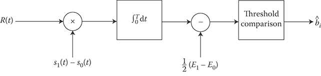
FIGURE 15.1 Optimal correlation receiver structure for binary communications.

Images

FIGURE 15.2 Optimal matched filter receiver structure for binary communications. In this case h(t) = s₁(T − t) − s₀(t − t).

By applying Equation 15.9 to 15.8 the final receiver structure is then given by

\int_{0}^{T} R (t) [s_{1} (t) - s_{0} (t)] d t - \frac{1}{2} (E_{1} - E_{0}) \begin{matrix} H_{1} \\ > \\ < \\ H_{0} \end{matrix} \frac{N_{0}}{2} ln \frac{π_{0}}{π_{1}} (15.10)

$\int_{0}^{T} R (t) [s_{1} (t) - s_{0} (t)] d t - \frac{1}{2} (E_{1} - E_{0}) \begin{matrix} H_{1} \\ > \\ < \\ H_{0} \end{matrix} \frac{N_{0}}{2} ln \frac{π_{0}}{π_{1}} (15.10)$

where E₁ and E₀ are the energies of signals s₁(t) and s₀(t), respectively. (See Figure 15.1 for a block diagram.) Importantly, if the signals are equally likely (π₀ = π₁), the optimal receiver is independent of the typically unknown spectral height of the background noise.

One can readily observe that the optimal binary communication receiver correlates the received waveform with the difference signal s₁(t) – s₀(t) and then compares the statistic to a threshold. This operation can be interpreted as identifying the signal waveform s_i(t) that best correlates with the received signal R(t). Based on this interpretation, the receiver is often referred to as the correlation receiver.

As an alternate means of implementing the correlation receiver, we may reformulate the computation of the left-hand side of Equation 15.10 in terms of standard concepts in filtering. Let h(t) be the impulse response of a linear, time-invariant (LTI) system. By letting h(t) = s₁(T − t) − s₀(T − t), then it is easily verified that the output of R(t) to an LTI system with impulse response given by h(t) and then sampled at time t = T gives the desired result. (See Figure 15.2 for a block diagram.) Since the impulse response is matched to the signal waveforms, this implementation is often referred to as the matched filter receiver.

15.5 Performance

On account of the nature of the statistics of the channel and the relative simplicity of the receiver, performance analysis of the optimal binary receiver in AWGN is a straightforward task. Since the conditional statistics of the log likelihood ratio are Gaussian random variables, the probability of error can be computed directly in terms of Marcum Q functions^* as

P_{e} = Q (\frac{∥ s_{0} - s_{1} ∥}{\sqrt{2 N_{0}}})

$P_{e} = Q (\frac{∥ s_{0} - s_{1} ∥}{\sqrt{2 N_{0}}})$

where the s_i are the two-dimensional signal vectors obtained from Equation 15.4, and where ‖x‖ denotes the Euclidean length of the vector x. Thus, ‖s₀ − s₁‖ is best interpreted as the distance between the respective signal representations. Since the Q function is monotonically decreasing with an increasing argument, one may recognize that the probability of error for the optimal receiver decreases with an increasing separation between the signal representations, that is, the more dissimilar the signals, the lower the P_e.

15.6 Signal Space

The concept of a signal space allows one to view the signal classification problem (receiver design) within a geometrical framework. This offers two primary benefits: first it supplies an often more intuitive perspective on the receiver characteristics (e.g., performance) and second it allows for a straightforward generalization to standard M-ary signaling schemes.

To demonstrate this, in Figure 15.3, we have plotted an arbitrary signal space for the binary signal classification problem. The axes are given in terms of the basis functions φ₁(t) and φ₂(t). Thus, every point in the signal space is a time function constructed as a linear combination of the two basis functions. By Fact 15.2, we recall that both signals s₀(t) and s₁(t) can be constructed as a linear combination of φ₁(t) and φ₂(t) and as such we may identify these two signals in this figure as two points.

Since the decision statistic given in Equation 15.8 is a linear function of the observed vector R which is also located in the signal space, it is easily shown that the set of vectors under which the receiver declares hypothesis H_i is bounded by a line in the signal space. This so-called decision boundary is obtained by solving the equation ln[L(R)] = 0. (Here again we have assumed equally likely hypotheses.) In the case under current discussion, this decision boundary is simply the hyperplane separating the two signals in signal space. Because of the generality of this formulation, many problems in communication system design are best cast in terms of the signal space, that is, signal locations and decision boundaries.

Images

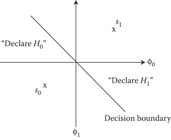
FIGURE 15.3 Signal space and decision boundary for optimal binary receiver.

*The Q function is the probability that a standard normal random variable exceeds a specified constant, that is, $Q (x) = \int_{x}^{\infty} 1 / \sqrt{2 π} \exp (- z^{2} / 2) d z .$ $Q (x) = \int_{x}^{\infty} 1 / \sqrt{2 π} \exp (- z^{2} / 2) d z .$

15.7 Standard Binary Signaling Schemes

The framework just described allows us to readily analyze the most popular signaling schemes in binary communications: amplitude-shift keying (ASK), frequency-shift keying (FSK), and phase-shift keying (PSK). Each of these examples simply constitute a different selection for signals s₀(t) and s₁(t).

In the case of ASK, s₀(t) = 0, while $s_{1} (t) = \sqrt{2 E / T} \sin (2 π f_{c} t)$ $s_{1} (t) = \sqrt{2 E / T} \sin (2 π f_{c} t)$ , where E denotes the energy of the waveform and f_c denotes the frequency of the carrier wave with f_cT being an integer. Because s₀(t) is the null signal, the signal space is a one-dimensional vector space with $ϕ_{1} (t) = \sqrt{2 / T} sin(2 π f_{c} t)$ $ϕ_{1} (t) = \sqrt{2 / T} sin(2 π f_{c} t)$ . This, in turn, implies that $‖ s_{0} - s_{1} ‖ = \sqrt{E}$ $‖ s_{0} - s_{1} ‖ = \sqrt{E}$ . Thus, the corresponding probability of error for ASK is

P_{e} (ASK) = Q (\sqrt{\frac{E}{2 N_{0}}})

$P_{e} (ASK) = Q (\sqrt{\frac{E}{2 N_{0}}})$

For FSK, the signals are given by equal amplitude sinusoids with distinct center frequencies, that is, $s_{i} (t) = \sqrt{2 E / T} \sin (2 π f_{i} t)$ $s_{i} (t) = \sqrt{2 E / T} \sin (2 π f_{i} t)$ with f_iT being two distinct integers. In this case, it is easily verified that the signal space is a two-dimensional vector space with $ϕ_{i} (t) = \sqrt{2 / T} sin(2 π f_{i} t)$ $ϕ_{i} (t) = \sqrt{2 / T} sin(2 π f_{i} t)$ resulting in $‖ s_{0} - s_{1} ‖ = \sqrt{2 E} .$ $‖ s_{0} - s_{1} ‖ = \sqrt{2 E} .$ The corresponding error rate is given to be

P_{e} (FSK) = Q (\sqrt{\frac{E}{N_{0}}})

$P_{e} (FSK) = Q (\sqrt{\frac{E}{N_{0}}})$

Finally, with regard to PSK signaling, the most frequently utilized binary PSK signal set is an example of an antipodal signal set. Specifically, the antipodal signal set results in the greatest separation between the signals in the signal space subject to an energy constraint on both signals. This, in turn, translates into the energy constrained signal set with the minimum P_e. In this case, the s_i(t) are typically given by $\sqrt{2 E / T} \sin [2 π f_{c} t + θ (i)]$ $\sqrt{2 E / T} \sin [2 π f_{c} t + θ (i)]$ , where θ(0) = 0 and θ(1) = π. As in the ASK case, this results in a one-dimensional signal space, however, in this case $‖ s_{0} - s_{1} ‖ = 2 \sqrt{E}$ $‖ s_{0} - s_{1} ‖ = 2 \sqrt{E}$ resulting in probability of error given by

P_{e} (PSK) = Q (\sqrt{\frac{2 E}{N_{0}}})

$P_{e} (PSK) = Q (\sqrt{\frac{2 E}{N_{0}}})$

In all three of the described cases, one can readily observe that the resulting performance is a function of only the signal-to-noise (SNR) ratio E/N₀. In the more general case, the performance will be a function of the intersignal energy to noise ratio. To gauge the relative difference in performance of the three signaling schemes, in Figure 15.4, we have plotted the P_e as a function of the SNR. Please note the large variation in performance between the three schemes for even moderate values of SNR.

Images

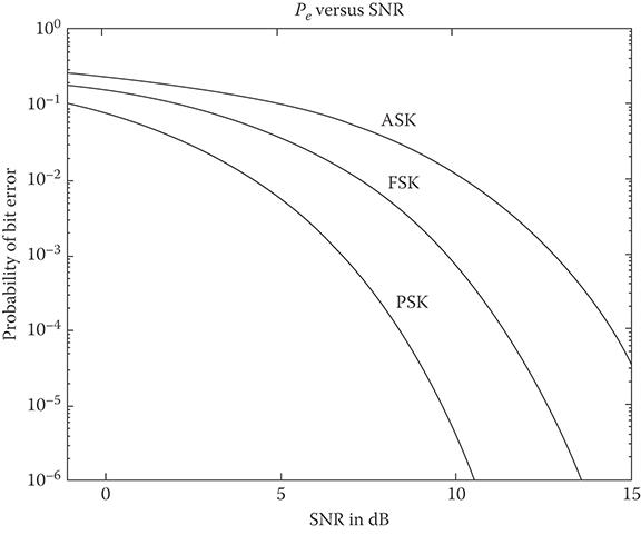
FIGURE 15.4 P_e versus the signal to noise ratio in decibels [dB = 10 log(E/N₀)] for amplitude-shift keying, frequency-shift keying, and phase-shift keying; note that there is a 3 dB difference in performance from ASK to FSK to PSK.

15.8 M-ary Optimal Receivers

In binary signaling schemes, one seeks to transmit a single bit over the bit interval [0, T]. This is to be contrasted with M-ary signaling schemes where one transmits multiple bits simultaneously over the so-called symbol interval [0, T]. For example, using a signal set with 16 separate waveforms will allow one to transmit a length four-bit sequence per symbol (waveform). Examples of M-ary waveforms are quadrature phase-shift keying (QPSK) and quadrature amplitude modulation (QAM).

The derivation of the optimum receiver structure for M-ary signaling requires the straightforward application of fundamental results in detection theory. As with binary signaling, the Karhunen–Loève expansion is the mechanism utilized to convert a hypotheses testing problem based on continuous waveforms into a vector classification problem. Depending on the complexity of the M waveforms, the signal space can be as large as an M-dimensional vector space.

By extending results from the binary signaling case, it is easily shown that the optimum M-ary receiver computes

ξ_{i} [R (t)] = \int_{0}^{T} s_{i} (t) R (t) d t - \frac{E_{i}}{2} + \frac{N_{0}}{2} \ln π_{i} i = 1, \dots, M

$ξ_{i} [R (t)] = \int_{0}^{T} s_{i} (t) R (t) d t - \frac{E_{i}}{2} + \frac{N_{0}}{2} \ln π_{i} i = 1, \dots, M$

where, as before, the s_i(t) constitute the signal set with the π_i being the corresponding a priori probabilities. After computing M separate values of ξ_i, the minimum probability of error receiver simply choose the largest amongst this set. Thus, the M-ary receiver is implemented with a bank of correlation or matched filters followed by choose-largest decision logic.

In many cases of practical importance, the signal sets are selected so that the resulting signal space is a two-dimensional vector space irrespective of the number of signals. This simplifies the receiver structure in that the sufficient statistics are obtained by implementing only two matched filters. Both QPSK and QAM signal sets fit into this category. As an example, in Figure 15.5, we have depicted the signal locations for standard 16-QAM signaling with the associated decision boundaries. In this case we have assumed an equally likely signal set. As can be seen, the optimal decision rule selects the signal representation that is closest to the received signal representation in this two-dimensional signal space.

Images

FIGURE 15.5 Signal space representation of 16-QAM signal set. Optimal decision regions for equally likely signals are also noted.

15.9 More Realistic Channels

As is unfortunately often the case, many channels of practical interest are not accurately modeled as simply as an AWGN channel. It is often that these channels impose nonlinear effects on the transmitted signals. The best example of this is channels that impose a random phase and random amplitude onto the signal. This typically occurs in applications such as in mobile communications, where one often experiences rapidly changing path lengths from source to receiver.

Fortunately, by the judicious choice of signal waveforms, it can be shown that the selection of the φ_i in the Karhunen–Loève transformation is often independent of these unwanted parameters. In these situations, the random amplitude serves only to scale the signals in signal space, whereas the random phase simply imposes a rotation on the signals in signal space.

Since the Karhunen–Loève basis functions typically do not depend on the unknown parameters, we may again convert the continuous time classification problem to a vector channel problem where the received vector R is computed as in Equation 15.3. Since this vector is a function of both the unknown parameters (i.e., in this case amplitude A and phase ν), to obtain a likelihood ratio test independent of A and ν, we simply apply Bayes theorem to obtain the following form for the LRT:

L (R) = \frac{E [p_{R} | H_{1}, A, ν (R | H_{1}, A, ν)]}{E [p_{R} | H_{0}, A, ν (R | H_{0}, A, ν)]} \begin{matrix} H_{1} \\ > \\ < \\ H_{0} \end{matrix} \frac{π_{0}}{π_{1}}

$L (R) = \frac{E [p_{R} | H_{1}, A, ν (R | H_{1}, A, ν)]}{E [p_{R} | H_{0}, A, ν (R | H_{0}, A, ν)]} \begin{matrix} H_{1} \\ > \\ < \\ H_{0} \end{matrix} \frac{π_{0}}{π_{1}}$

where the expectations are taken with respect to A and ν, and where p_R|H_i, A, ν are the conditional probability density functions of the signal representations. Assuming that the background noise is AWGN, it can be shown that the LRT simplifies to choosing the largest amongst

\begin{array}{r} ξ_{i} [R (t)] = π_{i} \int_{A, ν} \exp {\frac{2}{N_{0}} \int_{0}^{T} R (t) s_{i} (t | A, ν) d t - \frac{E_{i} (A, ν)}{N_{0}}} p_{A} (A, ν) d A d ν \\ i = 1, \dots, M \end{array} (15.11)

$\begin{array}{r} ξ_{i} [R (t)] = π_{i} \int_{A, ν} \exp {\frac{2}{N_{0}} \int_{0}^{T} R (t) s_{i} (t | A, ν) d t - \frac{E_{i} (A, ν)}{N_{0}}} p_{A} (A, ν) d A d ν \\ i = 1, \dots, M \end{array} (15.11)$

It should be noted that in the Equation 15.11 we have explicitly shown the dependence of the transmitted signals s_i on the parameters A and ν. The final receiver structures, together with their corresponding performance are, thus, a function of both the choice of signal sets and the probability density functions of the random amplitude and random phase.

15.9.1 Random Phase Channels

If we consider first the special case where the channel simply imposes a uniform random phase on the signal, then it can be easily shown that the so-called in-phase and quadrature statistics obtained from the received signal R(t) (denoted by R_I and R_Q, respectively), are sufficient statistics for the signal classification problem. These quantities are computed as

R_{I} (i) = \int_{0}^{T} R (t) \cos [2 π f_{c} (i) t] d t

$R_{I} (i) = \int_{0}^{T} R (t) \cos [2 π f_{c} (i) t] d t$

and

R_{Q} (i) = \int_{0}^{T} R (t) \sin [2 π f_{c} (i) t] d t

$R_{Q} (i) = \int_{0}^{T} R (t) \sin [2 π f_{c} (i) t] d t$

where in this case the index i corresponds to the center frequencies of hypotheses H_i, (e.g., FSK signaling). As in Figure 15.6, the optimum binary receiver selects the largest from amongst

ξ_{i} [R (t)] = π_{i} \exp (- \frac{E_{i}}{N_{0}}) I_{0} [\frac{2}{N_{0}} \sqrt{R_{I}^{2} (i) + R_{Q}^{2} (i)}] i = 1, \dots, M

$ξ_{i} [R (t)] = π_{i} \exp (- \frac{E_{i}}{N_{0}}) I_{0} [\frac{2}{N_{0}} \sqrt{R_{I}^{2} (i) + R_{Q}^{2} (i)}] i = 1, \dots, M$

where I₀ is a zeroth-order, modified Bessel function of the first kind. If the signals have equal energy and are equally likely (e.g., FSK signaling), then the optimum receiver is given by

Images

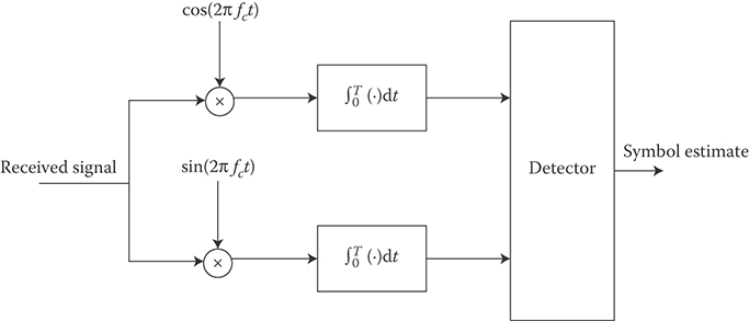
FIGURE 15.6 Optimum receiver structure for noncoherent (random or unknown phase) ASK demodulation.

R_{I}^{2} (1) + R_{Q}^{2} (1) \begin{matrix} H_{1} \\ > \\ < \\ H_{0} \end{matrix} R_{I}^{2} (0) + R_{Q}^{2} (0)

$R_{I}^{2} (1) + R_{Q}^{2} (1) \begin{matrix} H_{1} \\ > \\ < \\ H_{0} \end{matrix} R_{I}^{2} (0) + R_{Q}^{2} (0)$

One may readily observe that the optimum receiver bases its decision on the values of the two envelopes of the received signal $\sqrt{R_{I}^{2} (i) + R_{Q}^{2} (i)}$ $\sqrt{R_{I}^{2} (i) + R_{Q}^{2} (i)}$ and, as a consequence, is often referred to as an envelope or square-law detector. Moreover, it should be observed that the computation of the envelope is independent of the underlying phase of the signal and is as such known as a noncoherent receiver.

The computation of the error rate for this detector is a relatively straightforward exercise resulting in

P_{e} (noncoherent) = \frac{1}{2} \exp (- \frac{E}{2 N_{0}})

$P_{e} (noncoherent) = \frac{1}{2} \exp (- \frac{E}{2 N_{0}})$

As before, note that the error rate for the noncoherent receiver is simply a function of the SNR.

15.9.2 Rayleigh Channel

As an important generalization of the described random phase channel, many communication systems are designed under the assumption that the channel introduces both a random amplitude and a random phase on the signal. Specifically, if the original signal sets are of the form s_i(t) = m_i(t) cos(2πf_ct) where m_i(t) is the baseband version of the message (i.e., what distinguishes one signal from another), then the so-called Rayleigh channel introduces random distortion in the received signal of the following form:

s_{i} (t) = A m_{i} (t) \cos (2 π f_{c} t + ν)

$s_{i} (t) = A m_{i} (t) \cos (2 π f_{c} t + ν)$

where the amplitude A is a Rayleigh random variable^* and where the random phase ν is uniformly distributed between zero and 2π.

*The density of a Rayleigh random variable is given by p_A(a) = a/σ² exp(−a²/2σ²) for a ≥ 0.

To determine the optimal receiver under this distortion, we must first construct an alternate statistical model for s_i(t). To begin, it can be shown from the theory of random variables [4] that if X_I and X_Q are statistically independent, zero mean, Gaussian random variables with variance given by σ², then

A m_{i} (t) \cos (2 π f_{c} t + ν) = m_{i} (t) X_{I} \cos (2 π f_{c} t) + m_{i} (t) X_{Q} \sin (2 π f_{c} t)

$A m_{i} (t) \cos (2 π f_{c} t + ν) = m_{i} (t) X_{I} \cos (2 π f_{c} t) + m_{i} (t) X_{Q} \sin (2 π f_{c} t)$

Equality here is to be interpreted as implying that both A and ν will be the appropriate random variables. From this, we deduce that the combined uncertainty in the amplitude and phase of the signal is incorporated into the Gaussian random variables X_I and X_Q. The in-phase and quadrature components of the signal s_i(t) are given by $s_{I i} (t) = m_{i} (t) \cos (2 π f_{c} t)$ $s_{I i} (t) = m_{i} (t) \cos (2 π f_{c} t)$ and $s_{Q i} (t) = m_{i} (t) \sin (2 π f_{c} t)$ $s_{Q i} (t) = m_{i} (t) \sin (2 π f_{c} t)$ , respectively. By appealing to Equation 15.11, it can be shown that the optimum receiver selects the largest from

ξ_{i} [R (t)] = \frac{π_{i}}{1 + \frac{2 E_{i}}{N_{0}} σ^{2}} \exp [\frac{σ^{2}}{\frac{1}{2} + \frac{E_{i}}{N_{0}} σ^{2}} ({〈 R (t), s_{I i} (t) 〉}^{2} + {〈 R (t), s_{Q i} (t) 〉}^{2})]

$ξ_{i} [R (t)] = \frac{π_{i}}{1 + \frac{2 E_{i}}{N_{0}} σ^{2}} \exp [\frac{σ^{2}}{\frac{1}{2} + \frac{E_{i}}{N_{0}} σ^{2}} ({〈 R (t), s_{I i} (t) 〉}^{2} + {〈 R (t), s_{Q i} (t) 〉}^{2})]$

where the inner product

〈 R (t), S_{i} (t) 〉 = \int_{0}^{T} R (t) s_{i} (t) d t

$〈 R (t), S_{i} (t) 〉 = \int_{0}^{T} R (t) s_{i} (t) d t$

Further, if we impose the conditions that the signals be equally likely with equal energy over the symbol interval, then optimum receiver selects the largest amongst

ξ_{i} [R (t)] = \sqrt{{〈 R (t), s_{I_{i}} (t) 〉}^{2} + {〈 R (t), s_{Q_{i}} (t) 〉}^{2}}

$ξ_{i} [R (t)] = \sqrt{{〈 R (t), s_{I_{i}} (t) 〉}^{2} + {〈 R (t), s_{Q_{i}} (t) 〉}^{2}}$

Thus, much like for the random phase channel, the optimum receiver for the Rayleigh channel computes the projection of the received waveform onto the in-phase and quadrature components of the hypothetical signals. From a signal space perspective, this is akin to computing the length of the received vector in the subspace spanned by the hypothetical signal. The optimum receiver then chooses the largest amongst these lengths.

As with the random phase channel, computing the performance is a straightforward task resulting in (for the equally likely, equal energy case)

P_{e} (Rayleigh) = \frac{\frac{1}{2}}{(1 + \frac{E σ^{2}}{N_{0}})}

$P_{e} (Rayleigh) = \frac{\frac{1}{2}}{(1 + \frac{E σ^{2}}{N_{0}})}$

Interestingly, in this case the performance depends not only on the SNR, but also on the variance (spread) of the Rayleigh amplitude A. Thus, if the amplitude spread is large, we expect to often experience what is known as deep fades in the amplitude of the received waveform and as such expect a commensurate loss in performance.

15.10 Dispersive Channels

The dispersive channel model assumes that the channel not only introduces AWGN but also distorts the signal through a filtering process. This model incorporates physical realities such as multipath effects and frequency selective fading. In particular, the standard model adopted is depicted in the block diagram given in Figure 15.7. As can be seen, the receiver observes a filtered version of the signal plus AWGN. If the impulse response of the channel is known, then we arrive at the optimum receiver design by applying the previously presented theory. Unfortunately, the duration of the filtered signal can be a complicating factor. More often than not, the channel will increase the duration of the transmitted signals, hence, leading to the description, dispersive channel.

However, if the designers take this into account by shortening the duration of s_i(t) so that the duration of $s_{i}^{*} (t)$ $s_{i}^{*} (t)$ is less than T, then the optimum receiver chooses the largest amongst

ξ_{i} (R (t)) = \frac{N_{0}}{2} \ln π_{i} + 〈 R (t), s_{i}^{*} (t) 〉 - \frac{1}{2} E_{i}^{*}

$ξ_{i} (R (t)) = \frac{N_{0}}{2} \ln π_{i} + 〈 R (t), s_{i}^{*} (t) 〉 - \frac{1}{2} E_{i}^{*}$

If we limit our consideration to equally likely binary signal sets, then the minimum P_e matches the received waveform to the filtered versions of the signal waveforms. The resulting error rate is given by

P_{e} (d i s p e r s i v e) = Q (\frac{‖ s_{0}^{*} - s_{0}^{*} ‖}{\sqrt{2 N_{0}}})

$P_{e} (d i s p e r s i v e) = Q (\frac{‖ s_{0}^{*} - s_{0}^{*} ‖}{\sqrt{2 N_{0}}})$

Thus, in this case the minimum P_e is a function of the separation of the filtered version of the signals in the signal space.

The problem becomes substantially more complex if we cannot ensure that the filtered signal durations are less than the symbol lengths. In this case we experience what is known as intersymbol interference (ISI). That is, observations over one symbol interval contain not only the symbol information of interest but also information from previous symbols. In this case we must appeal to optimum sequence estimation [5] to take full advantage of the information in the waveform. The basis for this procedure is the maximization of the joint likelihood function conditioned on the sequence of symbols. This procedure not only defines the structure of the optimum receiver under ISI but also is critical in the decoding of convolutional codes and coded modulation. Alternate adaptive techniques to solve this problem involve the use of channel equalization.

Images

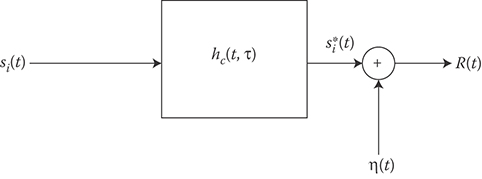
FIGURE 15.7 Standard model for dispersive channel. The time-varying impulse response of the channel is denoted byh_c(t, τ).

References

1. Gibson, J. D., Principles of Digital and Analog Communications, 2nd ed. New York: MacMillan. 1993.

2. Haykin, S., Communication Systems, 3rd ed. New York: John Wiley & Sons. 1994.

3. Lee, E. A. and Messerschmitt, D. G., Digital Communication. Norwell, MA: Kluwer Academic Publishers. 1988.

4. Papoulis, A., Probability, Random Variables, and Stochastic Processes, 3rd ed. New York: McGraw-Hill. 1991.

5. Poor, H. V., An Introduction to Signal Detection and Estimation. New York: Springer-Verlag. 1988.

6. Proakis, J. G., Digital Communications, 2nd ed. New York: McGraw-Hill. 1989.

7. Shiryayev, A. N., Probability. New York: Springer-Verlag. 1984.

8. Sklar, B., Digital Communications, Fundamentals and Applications. Englewood Cliffs, NJ: Prentice Hall. 1988.

9. Van Trees, H. L., Detection, Estimation, and Modulation Theory, Part I. New York: John Wiley & Sons. 1968.

10. Wong, E. and Hajek, B., Stochastic Processes in Engineering Systems. New York: Springer-Verlag. 1985.

11. Wozencraft, J. M. and Jacobs, I., Principles of Communication Engineering (Reissue), Prospect Heights, Illinois: Waveland Press. 1990.

12. Ziemer, R. E. and Peterson, R. L., Introduction to Digital Communication, New York: Macmillan. 1992.

Table of Contents for
15 Optimum Receivers

15

Optimum Receivers

15.1 Introduction

15.2 Preliminaries

15.3 Karhunen–Loève Expansion

15.4 Detection Theory

15.5 Performance

15.6 Signal Space

15.7 Standard Binary Signaling Schemes

15.8 M-ary Optimal Receivers

15.9 More Realistic Channels

15.9.1 Random Phase Channels

15.9.2 Rayleigh Channel

15.10 Dispersive Channels

References

Further Reading

Table of Contents for 15 Optimum Receivers

Create new playlist

Sign In

Sign Up

15

Table of Contents for
15 Optimum Receivers