
Soil mechanics and earthen construction: strength and mechanical behaviour
Abstract:
This chapter covers selected topics in mechanics and soil mechanics, which are important for an appreciation and understanding of the mechanical and hydraulic behaviour of unstabilised earthen construction materials. Stabilised materials are not covered in detail in this chapter, but aspects of their behaviour are clearly linked to those of unstabilised materials. The role of water is crucial as is the acceptance that many of the materials with which we are concerned are what is termed ‘unsaturated’.
8.1 Introduction
Understanding how earthen construction materials deform and carry loads is important in the development of design rules. For unstabilised earthen construction materials, the inherent properties of the soil mixture are of major significance. ‘Soil mechanics’ is the study of the fundamental principles governing the behaviour of all subsoil, and is a branch of civil engineering (subsoil being the ‘earth’ we are interested in, as opposed to topsoil, which we do not use for building). Soil mechanics principles are used by engineers designing foundations and retaining walls and for assessing the stability of slopes.
In this chapter some of the background necessary to understand the sources of strength in earthen construction materials will be covered. We will be focusing on unstabilised materials where strength derives from the properties of the earth mixture rather than from cementation supplied by a stabiliser (such as cement in modern stabilised rammed earth), however many aspects of the behaviour of stabilised materials are linked to these properties. To do this we will use the engineering science of ‘soil mechanics’, a discipline that emerged in the 1930s, which has since proved highly successful as a tool for civil and geotechnical engineers involved in designing foundations, retaining walls, tunnels, etc., in fact anything built in, on or with soil. Soil mechanics is also a vibrant area of research in many universities. It is important to state at the start that the soil in soil mechanics is subsoil, does not contain organic matter (unlike topsoil) and is the ‘earth’ used in earthen construction.
Basic mechanics is the foundation from which soil mechanics has developed and many complex soil behaviours can be understood using relatively simple mechanical concepts as will be demonstrated. The fundamental difference between soil and other civil engineering materials is that it is multi-phase, comprising soil grains and water. The changing balance between these components is the key to explaining its mechanical behaviour, and the simple concept of ‘effective stress’, which follows from recognition of this multi-phase nature, and which will be explained below, has proved of great power in development of methods for predicting movements and failure of geotechnical structures. While it is increasingly possible to measure the strength of soils in situ the majority of strength parameters used in calculations by engineers are obtained from laboratory tests on small samples of soils. In these tests the conditions in the ground, due to the presence of surrounding soil and changing water conditions, are mimicked as closely as possible.
Since the 1990s a subset of soil mechanics has grown up, termed unsaturated soil mechanics, in which it is recognised that many soils are three-phase, having air present in voids as well as water. This seemingly innocuous difference leads to wildly different behavioural features. It will be shown that many, if not all, modern unstabilised earthen construction materials can be regarded in part at least as manufactured unsaturated soils. For many stabilised materials, free water may also be present and therefore these could be regarded as cemented unsaturated soils. And therefore if we wish to build confidently with these materials we must also understand unsaturated soil mechanics.
8.2 Basic mechanics
Some basic mechanics is required to be restated so that the concepts to be discussed later are clear. Engineering mechanics can be divided into statics and dynamics. In the latter we consider problems in which there is acceleration, such as design of structures to withstand earthquakes, or the determination of the vibration modes of a bridge. In statics we consider that no acceleration is involved and the basic check is one of equilibrium, i.e. the principle that all the forces at a point which is not accelerating sum (in a vector sense) to zero. Statics and dynamics are not separate concepts, but together are Newton’s second law; in statics we have no inertial forces since there is no acceleration. As well as making sure that equilibrium is satisfied we have also to check compatibility (the notion that objects subject to loads deform smoothly), the boundary conditions are met (the points of support of the object and the loads applied to it) and finally the constitutive relation is followed. In statics we tend to be either dealing with one of two different situations: (i) what is happening at a point in a piece of material, and (ii) what is happening to a structure built out of various components. In this chapter we will be considering the first of these. Given a structure subject to loads, one of the most significant jobs of the engineer is to check conditions at material points within to assess likelihood of material failure.
8.2.1 The constitutive relation
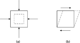
The link between the effects of the applied loads and the deformations produced at a material point is known as the constitutive relation. Loads and deformations are scale-dependent and we instead write constitutive relations in terms of their scale-independent counterparts, stresses and strains. By ‘effects’ here we do not mean the resulting deformations but the stresses produced in the material by the loads. Stress is a quantity calculated as force divided by area (so stress increases if we either increase the force or decrease the area over which it acts). Stress is often measured in civil engineering in units of Pascals (Pa) where 1 Pa = 1 Newton per metre squared (m2), and is usually given the Greek letter σ. We further classify stresses into normal and shear stresses. A normal stress is directed at right angles to the plane on which it acts, while a shear stress acts parallel to the plane. The difference between the two types of stress is illustrated in Fig. 8.1, which shows a rectangular block subjected to just shear stresses and just normal stresses. In the former the block is seen to change shape but not area. In the latter the situation is reversed. Note that Fig. 8.1a shows normal compressive stresses; stresses in the opposite directions, tending to stretch are termed tensile. For most materials it is shearing that leads to failure, and so we are most concerned with determining the maximum values of shear stress that can be experienced at a material point. The state of stress at a material point is visualised by thinking of an infinitesimally small cube placed at the material point whose sides are subject to normal and shear stresses. For each face of the cube there is one normal stress and two shear stresses, so for the whole cube there are 18 different stresses. However due to equilibrium only six of these stresses are different. Strain, in its simplest form, is a dimensionless ratio of a change in a dimension over the original dimension measured and is given the Greek letter ε. In a one-dimensional problem, such as the extension of a uniform rod, there is a single strain (the axial strain) calculatedss as
The constitutive relation links stresses to strains via the material properties where for each stress on the infinitesimal cube mentioned above there is a strain. In most real calculations we have to consider the full combination of stresses and strains acting at a point in all three dimensions, rather than being able to use a single stress as in the example above, a complex task that will not be covered in detail here.
The simplest constitutive relation is linear elasticity in which there are two material properties, usually taken as Young’s modulus, E, which is a measure of the stiffness of the material and Poisson’s ratio, ν, which is a measure of how much something deforms in one direction when loaded in another direction. For instance, taking a small block of clay and squashing it leads to deformations in directions at right-angles to the direction of squash. This is what most materials do and is an indication of a positive Poisson’s ratio. For the case of a material loaded in one direction only such as the rod in Fig. 8.2a Young’s modulus can be measured as
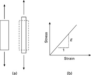
8.2 Young’s modulus in one-dimension (a) one-dimensional test of a loaded rod; (b) elastic stress–strain curve.
where σ and ε are the axial stress and strain respectively. If the stress–strain relationship is plotted then Fig. 8.2b is produced and Young’s modulus can be seen as the slope of the line. Table 8.1 gives Young’s modulus values for a number of civil engineering materials (the units are gigapascals, i.e. 1 GPa = 109 Pa). Two out of four material properties can be used for linear elasticity; instead of E and ν we sometimes replace one or both of these with bulk modulus K or shear modulus G where the conversions are:
Table 8.1
Young’s moduli for a range of materials
| Material | Young’s Modulus (GPa) |
| Steel | 205 |
| Aluminium | 70 |
| Aluminium | 15–45 |
| Brick | 10–20 |
| Soil | 0.3–10 |
| Rock | 1–100 |
Linear elasticity predicts (i) that the stress in the material is always proportional to the strain, (ii) that a material will continue to deform with increasing load forever and (iii) that on release of the load the deformation will entirely disappear. The second of these is clearly not realistic as materials fail, that is they either (i) reach a point where no more load can be applied and permanent deformations occur (which stay once the load is removed, known as ductile failure or yield) or (ii) the material fractures (known as brittle failure). Instead of the stress–strain behaviour looking like Fig. 8.2b plots look more like those in Fig. 8.3. Soils actually show very little elasticity, exhibiting permanent deformation (termed plastic) almost immediately upon loading. Therefore any useful constitutive relation must also include definition of the point of failure. E and ν, are lumped together as stiffness properties (i.e. how much and what type of deformation occurs for a given load). The properties and rules that tell us about failure are associated with strength. Understanding this distinction is vital in mechanics of materials. For materials such as metals, we often talk of a yield strength, which is a single stress beyond which the material can be expected to experience permanent (or plastic) deformation. In fact it is only for a very limited series of loading situations that one can directly compare a single yield stress with a single value of stress one calculates as occurring in the material. In modelling continuum materials, as we do in soil mechanics, the strength rules (often called yield or failure criteria) are written in terms of all stresses acting at a point (on the infinitesimal cube) considering all three dimensions.
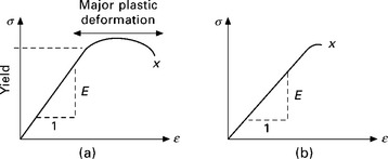
Brittle failure (Fig. 8.3b) is characterised as sudden fracturing with very little apparent plastic deformation; glass being a classic brittle material. Analysis of brittle failure is more complex than the ductile failure described above, largely because the process of brittle failure involves a sudden transfer of energy. Engineering fracture analysis tends to focus on the assumption of cracks of a certain length being present in a material and then answering the question: will those cracks get larger (propagate)? The material property most commonly used to assess this in metals is the fracture toughness KIC; a value that is compared to a stress intensity factor calculated using the applied stresses. This is a complex procedure to consider applying to non-metallic materials and is not considered in this way for soils and rocks. Instead a simpler approach is sometimes taken so that cracking is assumed to occur when the soil is subjected to tensile stresses (soil often being assumed to have no tensile strength).
For earthen construction materials we are almost always focused on strength rather than stiffness. While structures built from earth will deform due to applied loads (mostly due to the weight of the earth itself) these movements are generally insignificant and we are mostly concerned with the likelihood of failure. Therefore in what follows we will focus on strength, its sources and its measurement in these materials.
8.3 Fundamental soil behaviour
What distinguishes soil behaviour from other civil engineering materials? Examples are quite easy to point to. A soil slope can fail both due to being overloaded and due to rainfall. What is happening here? Would we consider a concrete structure (where particles are cemented together throughout) to behave any differently when wet than dry? The key mechanical concept in soil strength is friction and both of the slope failures can be explained by considering this physical phenomenon. The other major distinguishing feature of soil is that it is a multi-phase material, i.e. it contains soil grains, water and sometimes in addition, air. When it contains only soil grains and water it is termed saturated (i.e. all the voids in the soil are filled with water) and this is assumed to be so in the majority of cases considered by engineers in design. Two commonly used measures of soil state are usefully stated at this point. Firstly, the degree of saturation of a soil sample is given by:
where Vw is the volume of water and Vv is the volume of voids (i.e. Sr = 1 means full saturation). Water content is defined as:
where mw is the mass of water in a sample and ms is the mass of solids in the sample.
It is now widely accepted that friction holds soils together, but before applying this idea to soils we should consider simpler models of friction of the type studied at school. Consider a block sitting on a flat plane (Fig. 8.4). The block is subjected to a horizontal force F but will move only when F exceeds a certain value determined as:
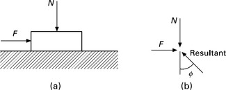
where μ is the coefficient of friction (a material property of the interface between block and plane) and N is the normal force across the plane, perhaps resulting from the block’s self-weight. The coefficient of friction can be replaced with the tangent of an angle ϕ as follows
where the angle is that made by the line of action of the reaction force from the plane to the vertical. As the normal force is increased so the frictional resistance to movement increases. As stated above, the majority of failures in materials are due to shear strength being exceeded, and we can easily see that the interface between the block and the plane is in shear, so that this frictional model is itself a model of shear strength. The first slope failure mentioned above occurs due to overloading leading to shear stresses in the slope exceeding the shear strength. The rainfall-induced failure cannot however be explained in the same way as the applied load has not changed so the shear stresses in the slope must be the same. The explanation is a little more subtle and requires the concept of effective stress.
8.4 Effective stress
The most powerful idea in traditional soil mechanics is that of effective stress, first proposed by an Austrian Engineer, Karl Terzaghi in the 1920s, which has never proved to be wrong ever since. The concept of effective stress lies behind all the geotechnical construction that surrounds us. The easiest way to understand effective stress is by reference to an idealised view of what is happening at the grain level in a soil (Fig. 8.5). The applied loads are now termed the total stress σ. These are the stresses that we check against equilibrium and are applied to the soil. Within the water there will be a pressure which we call the pore water pressure u. The total stress will be pushing the soil grains together while the pore water pressure will be pushing them apart. Remembering that pressure is the same thing as a stress, the difference between the two is called the effective stress σ′where
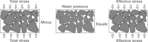
Effective stress is the stress transmitted through the arrangement of grains and is therefore the stress that will control the frictional behaviour. Crucially, Equation 8.8 shows that the effective stress can be altered both by changing the loads applied or by changing the water conditions. This now explains how soils can fail both by an increase in load but also by changes in the water pressures, as in the rainfall-induced landslide example above. The first increases the applied shear stress beyond the limit of the material; the second decreases the strength of the material by weakening the frictional capacity between grains. So the strength rules we write for soils have to be written in terms of the effective stresses not the total stresses.
Since it is now clear that the water in between the grains in a soil plays a crucial role in its behaviour it is worth explaining a pair of terms widely used in soil mechanics, which are also widely misunderstood, ‘drained’ and ‘undrained’. These terms refer to the conditions under which loads are applied to a soil sample, or soil at a location in the ground. Consider a sample of saturated soil loaded so that the pore water cannot escape. The applied load will be carried by an increase in the pore water pressure (the water is effectively incompressible as are the soil grains, so preventing volume change will increase the pressure). This is termed undrained loading. As we can see from Equation 8.8, this increase in pore water pressure will change the effective stress. Alternatively if the sample is free to lose water (but to still remain saturated throughout) then this is termed drained loading. Finegrained soils, such as clays, have very low permeabilities (which means that water cannot travel very fast since voids are tiny and tortuous). Therefore drained loading in these soils must be carried out very slowly; otherwise the pore water pressure will build up as it fails to travel through the void space fast enough, and if pore pressure changes so does effective stress. We can consider these loading conditions in design too. If a load is applied quickly to a clay soil the initial behaviour will be undrained, for instance. In fact undrained and drained loading are two ends of a spectrum of loading. In drained loading, water is leaving the sample so the sample volume must be reducing, and this volume change is known as consolidation. This is an important feature of soil behaviour considered by engineers in design as it tells them that soil constructions may continue to move (by consolidation) long after initial construction is finished, and determining the magnitude and time frame of these movements is critical in many cases. Two further terms that may also confuse are ‘normally consolidated’ and ‘overconsolidated’ which actually refer to current and previous states of effective stress. A normally consolidated material is at a yield point it has never before experienced. An overconsolidated sample has been unloaded from a normally consolidated state. Why this is important is that deformation behaviour differs markedly between the two classes. A famous example of an overconsolidated soil is the clay under most of north London (called London clay).
8.5 Models of shear strength for soils
The most commonly used strength ‘rule’ or yield criterion for soils is known as the Mohr-Coulomb criterion. This is a mathematical representation of the simple model of friction expressed in Equation 8.6. The angle ϕ’ is referred to as the effective angle of friction of the soil (since we are now concerned with effective stresses) and is a property that can be determined via a number of different soils tests. The superscript indicates we are dealing with effective stresses here (compare to Equation 8.7). Most commonly Mohr-Coulomb appears for the two-dimensional case as shown in Fig. 8.6 and can be expressed in terms of normal stress σ and shear stress τ as:
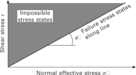
which is a statement of the stress state at failure, i.e. if the actual shear stress exceeds the value of the RHS of the equation then failure will occur. The Mohr-Coulomb criterion is related to drained loading. For undrained loading the shear strength is found to be independent of the normal stress and dependent only on the water content so that:
where cu is the undrained shear strength.
Many textbooks in the past, and even some today, include another term on the right-hand side of Equation 8.9 namely a cohesion c (or c′). This represents a strength inherent in the soil regardless of friction, i.e. some ‘glue’ holding the grains together. The notion that soil has an inherent strength available to it when the normal forces are zero is now recognised as incorrect for uncemented materials (it will however be present in stabilised earthen construction materials and some rocks). If there is no normal force at grain to grain contact, where is the frictional strength? In the past, supporters of cohesion have pointed to the electrostatic charges on clay particles as the source for this component, however analysis shows these forces to be an order of magnitude too low to be responsible. Others point to the visible evidence of standing clay faces in trenches as evidence of cohesion, however the reason for their stability (initially at least) lies in another mechanism entirely which will be considered in Section 8.8.
Beyond Mohr-Coulomb there is a wide range of advanced models for the shear strength of saturated soils. For the undrained case one can use models routinely used for metal plasticity (surprisingly) which have a single strength parameter, such as those due to Tresca and von Mises. For frictional behaviour by far the most popular models are based on the Critical State concept, a major advance in understanding the behaviour of soils developed at Cambridge University in the 1960s, which brings together shear strength with features of observed deformations and is most successful when applied to normally or lightly over-consolidated clays. Models suitable for stabilised earthen construction materials must include an additional source of strength from the interparticle bonding through cementation. These models have been developed for soils but are of considerably greater complexity than the models described above. For a lightly stabilised material, a considerable proportion of the strength behaviour may also be governed by friction.
8.5.1 Experimental methods for determination of strength
We have established that the primary mode of failure in soils, as in most other materials is that of shearing and that the strength parameters we wish to find for a soil are ϕ′or cu. We will now look at some of the most popular methods for determining strength parameters, whether these are required for the Mohr-Coulomb criterion described above or more complex models.
The shearbox test
Probably the simplest test is the direct shear (or shearbox) test which is explained in Fig. 8.7. The shear box test is mostly used for granular soils. The soil is placed or compacted into a small open chamber in the device and a vertical load is applied via a hanging weight applied through a grooved plate. The base of the device is then slowly displaced horizontally while the top half remains fixed thus shearing the sample. The horizontal load is measured (which gives the shear stress across the interface on division by the sample plan area) as well as the horizontal displacement. The peak shear stress divided by the normal stress gives the tangent of ϕ′from Equation 8.9. The test is repeated for a number of different normal stresses by emptying the box, refilling and using a different vertical load.
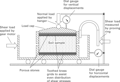
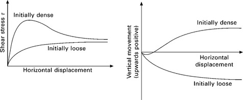
The vertical displacement of the hanging load is also measured and reveals another significant feature special to soils. Typical plots from shear box tests for materials in various states are shown in Fig. 8.8. where it can be seen that loose soils (i.e. those not compacted heavily into the chamber) show a downwards movement of the vertical load, while dense soils show an upwards movement of the vertical load and a peak strength that reduces to a residual level. So in shearing dense soils, the volume of the sample increases. This behaviour on yielding is unique to particulate materials and hints towards the idea that the soil is moving, in both cases, to a unique state where volume will not change, shearing will take place at a constant value of shear stress and, of course the normal stress will not change. This behaviour is one of the powerful features of Critical State Soil Mechanics and we can draw a parallel between loose samples in the shear box and normally consolidated clays, and between dense samples in the shear box and overconsolidated samples.
Triaxial tests
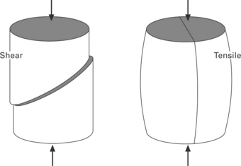
More complicated but of greater utility than the shearbox is the triaxial test where cylindrical samples surrounded by an impermeable membrane are placed in a chamber which is then filled with water, totally surrounding the sample. The sample is then squashed vertically at the same time as a constant pressure is applied via the water surrounding the sample. While it may not look as if this arrangement of loads is shearing in sense of the Fig. 8.1a it is still taking place since there is a difference between the stresses applied in the three different directions. Failure modes for these samples tend to fall into two classes, of shearing and barrelling as shown in Fig. 8.9. Triaxial testing provides much more information and control than the shear box test. It also does not force the sample to yield across a predefined plane, as happens in the shear box test. Triaxial tests are most easily carried out on clay materials since the cylindrical samples have to be self-supporting during preparation for the test, although there are techniques for carrying out these tests with sands. Drained and undrained tests are possible as the sample ends are supported on discs, which can be porous and linked to a drainage system. With the drainage tap turned off the water in the sample cannot escape and the test is therefore undrained. With the tap switched on a drained test can be carried out, although for the reasons above, this must usually be done very slowly. It is also relatively easy to include additional sensors in the triaxial test to monitor pore water pressures during shearing, and hence determine effective stresses. Complex triaxial testing equipment can be computer-controlled to subject samples to intricate stress paths.
Other tests
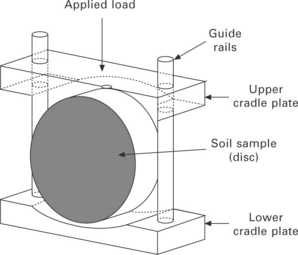
The shearbox and triaxial tests determine parameters for models of shear strength and also stiffness parameters if necessary. Determining the tensile strength of soils for the purposes of simple fracture prediction is very difficult, however this may be of major importance for stabilised materials and one simple test, borrowed from rock mechanics, can be used on soils which are either cemented slightly, or have tensile strength from a source to be discussed in Section 8.8. This is the Brazilian test. The testing arrangement is shown in Fig. 8.10 and comprises the loading of a thick disc of material thickness t across its diameter D to failure load P. The Poisson’s ratio effect means that the compressive loading across the diameter induces a tensile strain in the opposite direction, which causes the specimen to crack and via analysis one can link the failure load P to the approximate tensile stress acting horizontally at the centre of the disc σt as
The use of this test and development of equipment for earthen construction materials is further discussed in Beckett (2008).
8.6 Unsaturated soil behaviour
Terzaghi’s theory of effective stress applies only to saturated soils, i.e. those where water fills the inter-grain pores entirely. In many applications, however, the assumption of full saturation is incorrect. Even in temperate climates such as the UK, the top half-to one-metre of natural soil may not be fully saturated at certain times of the year. The water table may lower leaving a zone (known as the vadose zone) above which some water will remain by capillary action but air will be present in the pores too. In hotter parts of the world the upper layers of soil, where most engineering construction takes place, will be unsaturated. So, the question is, is this significant for soil mechanics? Can Terzaghi’s effective stress be adapted for use in unsaturated conditions? Before addressing these questions it is wise to consider the changes to mechanical behaviour on desaturation.
Unsaturated soils are known to be stronger than their saturated counterparts. This is easy to test yourself. Building sandcastles is an experiment in unsaturated soil mechanics. Completely dry sand is useless as a construction material, as is very wet sand. The former blows away while the latter tends towards a fluid (and fluids in the main cannot withstand shear stress so are not candidates for building materials). There is, however, somewhere in between when sand is just wet enough to make a good building material, for sandcastles anyway, and that is a condition where there is water and air in the voids between particles. This must be an unsaturated case as, if it were saturated, one would not be able to add any more water to the mixture, and clearly you can. So what is providing the additional shear strength in this unsaturated case?
8.6.1 Suction
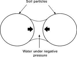
The explanation for this is ‘suction’. Consider two sand grains in an unsaturated soil. Water will be held in menisci between grains, with curved surfaces as shown in Fig. 8.11. Some simple physics tells us that because of the curvature of the menisci surfaces the pressure of the water inside the meniscus must be tensile, i.e. the opposite case to that we have discussed above for saturated soils. So, instead of the water pushing the grains apart it pulls them together and this effect will be heightened if the air pressure in the voids ua is not atmospheric. Therefore the normal frictional force at contacts is greater in the unsaturated case. A greater normal force leads to a greater frictional force and hence explains the greater shear strength. Suction is therefore defined as the difference between the air pressure and the pore water pressure, i.e. s = ua – uw. A tensile pore water pressure would appear as a negative quantity in this equation thus giving a positive value of suction.
Unsaturated soils have a number of other behavioural differences to saturated soils, but when considering earthen construction, suction is of most significance. It helps to explain why unstabilised earthen materials do not collapse, since while they may look dry they cannot be totally so. The small amount of water present provides suction to aid basic frictional shear strength. Constitutive modelling for unsaturated soils is an active area of research at present, but there is a lack of consensus as to what stress variables should be used to characterise strength. What is clear is that one cannot adopt Terzaghi’s effective stress (Equation 8.8) for unsaturated soils. Instead many researchers use net stress ![]() and suction. An example of a highly regarded model for unsaturated soils is the Barcelona Basic Model (BBM) developed by Alonso et al. (1990)
and suction. An example of a highly regarded model for unsaturated soils is the Barcelona Basic Model (BBM) developed by Alonso et al. (1990)
8.6.2 The soil water retention curve (SWRC)
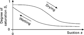
One other feature of unsaturated soil behaviour is worth mentioning as it is linked to the suction expected in a sample at a given water content, namely the soil water retention curve (SWRC). This is the relationship between suction and either the water content or degree of saturation of a sample. Typical curves for both drying and wetting are shown in Fig. 8.12. At saturation, suction is zero since the pore water pressure will be zero and there will be no air in the voids to supply ua. As a sample dries, water is lost and suction increases. This continues until the point where the remaining water is located in tiny quantities at grain contacts and around clay particles, and special techniques would be needed to entirely remove this water. This is the residual water content. If the sample is then wetted the path taken back to saturation is different, a hysteretic effect as shown in Fig. 8.12. This has consequences for the measurement of suctions as it is then a requirement to know if the sample was wetting or drying.
Mention has already been made of measurements of pore water pressures in the triaxial test and one question here is, can suctions be measured? The answer is sometimes, but not with great accuracy above a certain level of suction. Many devices have been developed, in universities, in the past 15 years to measure suction with varying degrees of success. High accuracy results up to suctions of 1.5 MPa can be made using small devices known as tensiometers (for examples see Lourenço et al., 2008; Tarantino and Mongiovi, 2001; Ridley and Burland, 1993). At higher suctions the options are limited but include the filter paper test and psychrometers (Rahardjo and Leong, 2006).
8.7 The use of soil mechanics in earthen construction
The preceding has covered the very basics of soil mechanics, which might be of relevance to those working with earthen construction materials. Other chapters in this book will cover stabilised materials in more detail and the means of design of various structural elements, such as foundations and retaining walls. For these types of construction the strength models outlined above will often still be of direct relevance, as part of the analysis will be to check the stability of the element itself, which will require assessment of the working stresses within and a comparison with the strength, which will in turn be based on the results of tests on small samples. For other structural members such as the use of highly stabilised earth to form beams and lintels, the emphasis on material point behaviour may be less immediately relevant although the coverage on fracture and tensile strength may be useful. Despite this, it seems obvious that those working with earth/soil should be aware of its fundamental properties and be able to explain behaviour, especially when things go wrong. The crucial role that water has to play in the strength of soils, with or without stabiliser, should be clear and hence the need for any designers in earth to be fully aware of this important aspect.
8.8 Future trends
The most vibrant area of soil mechanics research in universities is unsaturated soil mechanics and, worldwide, many researchers are working to develop new constitutive models, laboratory equipment and numerical modelling techniques. Centres of excellence in research are UPC (Barcelona), ENPC (Paris), and the Universities of Glasgow and Durham University in the UK. Considerable work is also ongoing attempting a more fundamental understanding of these materials at the microstructural level, using modern methods of non-intrusive investigation such as X-ray computed tomography (Hall et al., 2010). Earthen construction materials have only recently been recognised as manufactured unsaturated soils in works such as Jaquin et al. (2009) and Gelard et al. (2007), and the application of soil mechanics principles to these materials is at an early stage. The same can be said for the development of models for bonded unsaturated soils, of use for analysis of stabilised materials. The conservation of historical earthen construction is likely to be a major beneficiary from our improving geotechnical understanding of these materials, as stabilisation is likely to be absent or at a low level. A clear gap in knowledge is our understanding of fracture processes in dry earthen construction materials, but this area remains open in geotechnical engineering in general.
8.9 Sources of further information
There are many textbooks covering soil mechanics aimed at undergraduates on civil engineering courses. Most contain sections on soil strength, hydraulic behaviour and testing, as well as sections on design in/on/with soil. Recommended textbooks are those by Powrie (2002) and Smith (2006). Online one can access full texts on soil mechanics at the website of Professor Arnold Verruijt (http://geo.verruijt.net) and at the Géotechnique information site www.geotechnique.info/. Schofield (2005) is an interesting account of major misunderstandings in soil mechanics that have not yet been entirely banished, and Likos and Lu (2004) is a readable introduction to unsaturated soil mechanics. Soil mechanics research is published in journals such as Géotechnique, Computers and Geotechnics and the Institution of Civil Engineers Proceedings: Geotechnical Engineering.
8.10 References
Alonso, E.E., Gens, A., Josa, A. A constitutive model for partially saturated soils. Géotechnique. 1990; 40:405–430.
Beckett, C.T.S. Cracking in rammed earth, MEng dissertation. Durham: Durham University; 2008.
Gelard, D., Fontaine, L., Maximilien, S., Olagnon, C., Laurent, J., Houben, H., Van Damme, H., When physics revisits earth construction: recent advances in the understanding of the cohesion mechanisms of earthen materials. Proc. International Symposium on Earthen Structures. 2007. [IIS Bangalore, 22–24 August 2007, 294–299].
Hall, S.A., Bornert, M., Desrues, J., Pannier, Y., Lenoir, N., Viggiani, G., Besuelle, P. Discrete and continuum analysis of localised deformation in sand using X-ray μ CT and volumetric digital image correlation. Géotechnique. 2010; 60:315–322.
Jaquin, P.A., Augarde, C.E., Gallipoli, D., Toll, D.G. The strength of unstabilised rammed earth materials. Géotechnique. 2009; 59:487–490.
Likos, W.J., Lu, L. Unsaturated Soil Mechanics. London: John Wiley & Sons; 2004.
Lourenço, S.D.N., Gallipoli, D., Toll, D.G., Augarde, C.E., Evans, F.D., Medero, G.M. Calibrations of a high suction tensiometer. Géotechnique. 2008; 58:659–668.
Powrie, W. Soil Mechanics: Concepts and Applications, 2nd edition. Didcot: Taylor & Francis; 2002.
Rahardjo, H., Leong, E.C. Suction measurements. Geotechnical Special Publication (ASCE). 2006; 147:81–104.
Ridley, A.M., Burland, J.B. A new instrument for the measurement of soil moisture suction. Géotechnique. 1993; 43:321–324.
Schofield, A.N. Disturbed Soil Properties and Geotechnical Design. London: Thomas Telford; 2005.
Smith, I. Smith’s Elements of Soil Mechanics, 8th edition. Oxford: Wiley-Blackwell; 2006.
Tarantino, A., Mongiovi, L. Experimental procedures and cavitation mechanisms in tensiometer measurements. Geotechnical and Geological Engineering. 2001; 19:189–210.