
Chapter 9
Power Optimization
When embedded systems are either battery operated or deployed in large quantities, power usage is a primary concern in the design. Cost, performance, power, and size are the design considerations that must always be balanced in the design of a computer system.
In this chapter, we consider the power management features that are common to modern embedded computer system components, from CPU-specific features to platform-level industry standards for system management. Moreover, we illustrate a power optimization process that software engineers can use to manage the power efficiency of applications and systems software. While much of power management is handled in platform components, software design choices can have a considerable impact on overall power efficiency.
We begin the discussion with an overview of power consumption in electronics. We focus in particular on the principles that drive power efficiency.
Power Basics
Modern integrated circuits are manufactured with a complementary metal oxide semiconductor (CMOS) fabrication process. In a CMOS process, circuits are built with interconnected metal oxide semiconductor field effect transistors (MOSFETs). The power characteristics of these transistors dominate the power characteristics of modern digital electronics, including embedded systems.
Circuits of MOSFETs dissipate power actively by charging capacitors in the circuit network, and this charging happens every time the circuit switches. Active power can be modeled as P = CV 2 f, where C is the capacitive load, V is the voltage difference across the device, and f is the switching frequency.
Circuit designers have direct control over all three contributing factors, but the capacitive load is a consequence of the physical layout of the circuit and so cannot be managed or varied dynamically. Voltage and frequency, however, can both be changed throughout the operation of the circuit, although doing so requires a substantial circuit design effort.
It is possible to design circuits, and indeed entire logic devices such as CPUs, in order to vary operating voltage and frequency in response to system policy. For example, since voltage and frequency are both first-order determinants of performance, during idle times both can be reduced. When lower performance can be tolerated, opportunities arise to reduce power consumption.
Dynamic power is not the only form of power dissipation. Static power is also consumed in between transistor switching cycles. Historically, this leakage power has been negligible, but two trends have pushed it to the forefront. First, in order to accommodate high frequencies, designers typically utilize transistors that operate at voltages very near the switching threshold. This enables fast operation, but increases the fraction of time during which charge can leak across the device (that is, the so-called subthreshold leakage current). Second, modern submicron CMOS processes use very thin gate insulators that make it possible for current to tunnel through the insulator. In fact, the design of highly resistant gate materials is one of the most critical advances required to keep Moore’s Law on track, and recent processes have transitioned away from the use of the traditional gate dielectric, silicon dioxide, in favor of highly resistant dielectrics such as those based on hafnium. An operational system can manage leakage power by completely powering down circuits and by increasing threshold voltage (and this latter is at odds with reducing dynamic power).
Circuit designers and semiconductor process engineers have many years of innovation ahead in which they will further improve the power efficiency of integrated circuits. However, at any given time, system designers and programmers must understand the means at their disposal to influence and minimize power consumption. To do so, we now discuss the overall power context for an embedded system.
The Power Profile of an Embedded Computing System
Embedded systems are varied, and so are their power profiles. Some embedded systems are always powered on and provide continuous operation. Many types of displays, controllers, and networking devices have usage models that demand that they provide near-peak performance, nearly all of the time.
Other types of embedded computer systems have more variable workloads. Mobile handsets and mobile computers, for example, often have very bursty workloads that vary according to user behavior. With a varying workload comes an opportunity to vary the operational characteristics of the system. In user-facing mobile systems, for example, it is often possible for system components to “sleep” at sub-millisecond frequency in order to reduce overall power consumption without impacting the user experience. Given that humans cannot perceive visual change at frequencies above 60 Hz, opportunities exist to reduce or shut down the operation of system components at frequencies beyond human perception.
It is not surprising, then, that the bulk of advanced power management techniques and features has emerged first in mobile platforms. For example, Intel SpeedStep® technology was introduced in Pentium® M processors in order to support both policy and usage-based frequency and voltage control. The Windows™ operating system has supported Intel SpeedStep technology since its inception. The operating system and CPU work together effectively in a mobile context, such as a laptop. When operating from battery power, Intel SpeedStep technology is enabled and can be configured via operating system preferences to emphasize either performance or battery life (“Max Battery”). When Intel SpeedStep technology is enabled, both clock frequency and voltage are scaled down to reduce dynamic power consumption. Using the default settings, a user benefits from the presence of Intel SpeedStep technology as a natural consequence of plugging in or unplugging the laptop.
Of course, CPUs are not the only components found in a system. Historically, CPUs have been the most intensive consumers of power, but in recent years the growing importance of mobile computing has prompted increases in power efficiency and power management in mobile CPU products. For reasons unrelated to mobile computing and more related to cost-effective power dissipation and reducing the energy contribution to total cost of system ownership, server and desktop chips have experienced similar degrees of improvement in power efficiency. Non-mobile chipsets have certainly benefitted from many of the power efficiency and power management techniques developed for mobile systems.
While CPUs have improved considerably, other system components have been slower to increase power efficiency. With CPUs now consuming a smaller portion of the overall system power budget, manufacturers of other components, such as memory, displays, and I/O devices, have found an unmistakable reason to begin improving power efficiency in earnest.
The first challenge for any system component is to maximize the range of power consumption between low-power states and high-power ones. To see why, consider that it is only beneficial to manage power actively if substantial power savings are to be had, and that the only way for a system or component to achieve substantial power savings is for it to exhibit significantly lower power consumption when idle or under low utilization as compared to the power consumed under load. In other words, if the difference between minimum power and maximum power is negligible, then power management will have a negligible impact.
To clarify this idea, we now discuss the difference between constant and dynamic power in the context of an example system.
Constant versus Dynamic Power
When the hardware system components can operate in a range of power and performance states, from low-power and low-performance to high-performance and peak power, then the resulting power efficiency of an operational system becomes a consequence of the actions and activity of the operating system and application software. Software engineers would hope that idle software would lead to lower power consumption.
However, all systems have some degree of power consumption that is independent of system use. This constant power is drawn regardless of load.
Constant Power
An embedded computer consumes a constant, minimum amount of power when powered on, regardless of the level of system activity. Unfortunately, it is often the case that this constant power dominates the overall power budget of a system. Other than by powering a system down completely or transitioning to a sleep state, software cannot influence a system’s constant power.
Dynamic Power
If most of the components in an embedded system support low-power modes, then dynamic power consumption can be significantly controlled through the careful use of resources. An operating system may either observe load or receive explicit signals from applications in order to decide to transition the machine to a lower-power, and consequently lower-performance, state. However, any benefits associated with doing so must be measured against the background constant power that is always being drawn.
To make the discussion concrete, we begin with a discussion of a platform based on the Intel® Atom processor from CompuLab, the fit-PC2. The fit-PC2 is a small-form factor computer built around the 1.6-GHz Intel Atom Z530 CPU and the Intel US15W chipset. With 1 GB DRAM, a 160-GB hard drive, and a full array of I/O channels, including six USB ports, Gigabit Ethernet, and Wi-Fi™, the fit-PC2 offers a typical low-end computing platform in a very small form factor (4.5 x 3.9 x 1.1 inches, or 115 x 101 x 27 millimeters).
Figure 9.1 reports power data for the fit-PC2 in two columns. The first column indicates the power consumption of the platform as reported by the manufacturer. The column has two stacked components. The bottom component indicates the idle power consumption; that is, the power consumed when the system is not executing any user-level application or OS-based service or maintenance task. As can be seen, the reported idle power is 6 W. The top component is the corresponding value under load, reported to be 9 W.
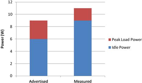
FIGURE 9.1 Advertised and Measured Dynamic Power Range for CompuLab’s fit-PC2. The Advertised Power Range Covers 66% of Peak, Whereas the Measured Value, When Accounting for Active I/O Devices, Covers 81% of the Observed Peak.
The second column indicates the idle and loaded power consumption as measured at the outlet (that is, by measuring “wall power”) on a test system running Ubuntu™ Linux. Such measurements can easily be gathered through the use of low-cost digital power meters. As the chart reports, the measured idle and loaded power consumption rates correspond to 9 W and 11 W, respectively. Given that the combined thermal design power (TDP) for the Intel Atom Z530 and its US15W chipset is 5 W, and that TDP for these chips represents fixed upper bounds on the power that will be dissipated by these two packages, we can see that a substantial fraction of power is consumed in non-CPU and non-chipset components.
The point of this exercise is not to call attention to the difference between the advertised and measured power values. Indeed, any estimates are expected to be loose because they are usually highly dependent on the type and number of I/O devices that are present in the system, such as hard disks and USB devices.
The main point of this figure is to point out the difference between the constant amount of power that will be consumed by such a system regardless of the load and the peak power consumption. It is constructive to consider the ratio between the two. The estimate has a ratio of idle to peak of 6/9 = 0.66, while the observed values correspond to a ratio of 9/11 = 0.81.
These ratios suggest that, say, 75% of total system power consumption is completely independent of software-level activity on this platform. If the system is powered up and capable of executing software, then it will consume at least 75% of its peak power regardless of the organization and activity of the application software and of the attempts at power management made by the operating system.
In other words, when the system has 0% utilization, it will consume 75% of its peak power. Clearly, the benefits of power management are limited in this platform. Intuitively, we desire a system that consumes power in proportion to its utilization.
The obvious problem with managing power efficiency in this platform is its comparatively large constant power consumption. In order to increase the effectiveness of dynamic power management, this constant power must be reduced. Even if the peak power is unchanged, a significant lowering of the constant power will enable software engineers to better manage the power efficiency of the system.
Indeed, future computer system designs aim to improve the effectiveness of dynamic power management in this way. To explore the impact of likely advances, we can construct and explore a simple model of efficiency.
A Simple Model of Power Efficiency
Suppose our system is capable of linearly scaling power consumption with utilization, or load. Given a fixed constant power, which is the power consumption observed at zero load, we can define our system’s power efficiency by taking the ratio of power usage to utilization.
Figure 9.2 illustrates an example with constant power equal to 50% of peak power. Thus, at 0% load, it consumes 50% of peak power for an efficiency of 0/50 = 0. At 10% load, since power consumption scales linearly with load in our model, normalized power consumption is 55%, yielding an efficiency of 18%. As illustrated in the figure, the system is highly inefficient over most of its operating range and does not achieve 80% efficiency until utilization rises to 70%. Note that we do not want efficiency to scale with load; rather, we would like high efficiency over the entire operating range. As we will see, our simple model suggests that a dramatically lower constant power has a transformative impact on the overall power efficiency of a system. In our fit-PC2 example, we saw that constant power represented around 80% of peak power, and Figure 9.2 represents a system with a constant power that corresponds to 50% of peak power. Future systems, however, may well have substantially lower constant power profiles.
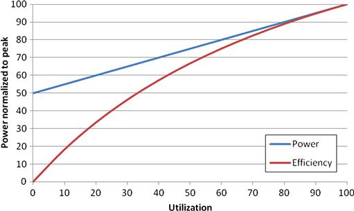
FIGURE 9.2 Power Consumption and Efficiency for a System With a Dynamic Power Range Down to 50% of Peak Performance. Power is Normalized to Peak Consumption. Efficiency is Calculated by Dividing Utilization by Normalized Power.
Figure 9.3 illustrates results for a system with a constant power that corresponds to 10% of peak power. As can be seen, the efficiency of the unloaded system necessarily remains 0%. However, at 10% load, the system exhibits efficiency of 52%! In fact, 80% efficiency is achieved at a load of 30%. At 50% utilization, the system is 90% efficient.

FIGURE 9.3 Power Consumption and Efficiency for a System With a Dynamic Power Range Down to 10% of Peak Performance. Power is Normalized to Peak Consumption. Efficiency is Calculated by Dividing Utilization by Normalized Power.
While current systems do not exhibit such low constant power, this is clearly the direction in which future system designs are heading.
It stands to reason that if an entire system is to be capable of a 10% constant power, then each major hardware component must be as well. Recall that in the fit-PC2, the Intel Atom Z530 and its US15W chipset consumed a maximum of 5 W of the peak observed 11 W of power. So more than half of peak power is contributed by non-CPU and non-chipset components.
This observation illustrates the need for comprehensive system efficiency and a power management scheme that manages power in all hardware components. However, consider the challenge involved with doing so. It is acceptable for an operating system to adapt its low-level systems software in order to accommodate the power management features of a CPU produced by companies like Intel, but only because there are so few types of CPUs that operating system vendors must be aware of! It is not so for memory and I/O device manufacturers.
So how can operating systems accommodate these non-CPU components? And, clearly, any power management scheme must be part of a strategy mediated by the operating system. For a component or device to substantially reduce its power consumption, it must be able to enter a sleep mode, and such a transition in the I/O subsystem must be apparent to the operating system for reasons of stability and performance.
To address this issue, which is in fact a reflection of the overall management requirement that must be sustained between an operating system and the system components, platform-specific industry standards have been developed that define the roles, responsibilities, and specific mechanisms provided to achieve reliable power management and system configuration.
In the next section, we introduce the current standard for managing power in computer systems, the Advanced Configuration and Power Interface (ACPI), which is used in computer systems of all scales to manage power and device configurations. ACPI represents the contemporary philosophy, and indeed the universal industrial standard among manufacturers, of how to manage power in computer systems.
Advanced Configuration and Power Interface (ACPI)
ACPI is a standard that has been developed through the cooperation of a group of companies in the computer industry: Hewlett-Packard, Intel, Microsoft, Phoenix Technologies, and Toshiba. The purpose of ACPI is to provide a standard interface for computer system power and configuration management. Through ACPI, the operating system is granted exclusive control over all system-level management tasks, including the boot sequence, device configuration, power management, and external event handling (such as thermal monitoring or power button presses).
ACPI is an evolutionary development that has drawn upon a collection of earlier technologies that individually managed specific tasks. Consequently, ACPI subsumes and replaces technologies such as plug-and-play BIOS, power management BIOS routines, Advanced Power Management (APM), and multiprocessor configuration APIs.
In these previous-generation designs, spreading system configuration and power management responsibility across several different technologies within a system makes it difficult both to optimize system and power management and to develop and exploit effective new management features in system hardware components. Furthermore, since these APIs are not generally interoperable, platform- and operating system–specific development must be undertaken in order to provide support for a wide range of motherboard designs. ACPI has been designed to eliminate this fragmentation and provide robust, efficient, and extensible platform and power management.
Figure 9.4 illustrates the relationship between ACPI, its major internal components, and the rest of a computer system. Entities in red are part of ACPI proper, and while the data held within the memory structures are specific to a platform and to a platform-instance, ACPI interfaces are used to communicate and interpret the meaning of the data.
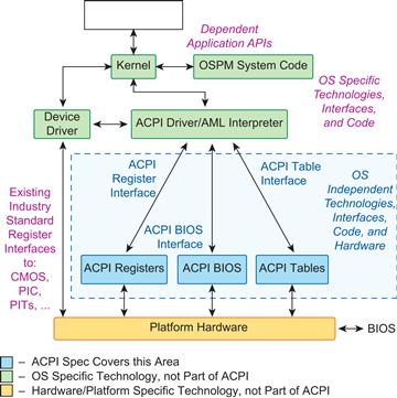
FIGURE 9.4 The Organization of ACPI in a Computer System. From the Advanced Configuration and Power Interface Specification, Revision 4.0.
As indicated in Figure 9.4, ACPI has three major components:
• ACPI Registers. These registers are well-defined locations that can be read and written to monitor and change the status of hardware resources.
• ACPI BIOS. This firmware manages system boot and transitions between sleep and active states. The ACPI tables are provided by the ACPI BIOS.
• ACPI Tables. These tables describe the interfaces to the underlying hardware and represent the system description. In order to keep hardware descriptions generic and extensible, a domain-specific language has been defined within ACPI. The language, known as the ACPI Machine Language (AML), is a compact, pseudo-code style of machine language. The operating system’s ACPI driver includes an interpreter for AML. In ACPI parlance, hardware descriptions are called Definition Blocks.
ACPI is a large specification, and most of its details are beyond the scope of this book. The most important aspect for embedded systems programmers to understand is how the ACPI management strategy relates to power optimization. To gain this understanding, we must consider the state-based model that ACPI employs to relate a system’s current state to the operating system and user-visible platform management goal.
Idle Versus Sleep
The two dominant forms of user-facing power management, idle and sleep, have different characteristics and motivations. Sleep states were introduced to allow laptop users to quickly power down a system and then power it up again without having to reboot the system from disk, which is a comparatively long-latency event. In sleep states, the system appears to be powered off completely, while in fact some software may periodically execute to service external events, such as network packet arrivals. Idle modes were introduced to take advantage of the variation in system utilization when the system is powered up. Transitions are made between idle modes at the granularity of seconds and less to reduce active power consumption; these transitions happen without the involvement or even awareness of the user.
ACPI develops these basic notions substantially.
ACPI System States
Figure 9.5 presents a high-level overview of how explicit states are used to implement an overall system management strategy. As can be seen, several types of related states are used to model the overall state of the system as well as the states of individual system components such as CPUs and I/O devices. The G states represent system state; within the sleep state G1, multiple levels of sleep are differentiated via S states. C states encode the state of CPUs; within state C0, P states distinguish between performance and power consumption levels. D states do the same for I/O devices. A uniform interpretation can be applied to the number scheme: the 0-level state always corresponds to a fully operational state, and the higher numbers indicate increasing deep sleep states with correspondingly lower power consumption and higher return latencies. We now briefly discuss each in turn.
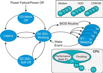
FIGURE 9.5 Relationship between Global, CPU, and Device States in ACPI. From the Advanced Configuration and Power Interface Specification, Revision 4.0.
Global System States (Gx States)
Global system states describe the entire system, and transitions between these states are typically obvious to the user.
G0: Working. In this state, the computer is in a normal operating mode, executing user application threads. As described next, the operating system can optionally manage the performance state of the CPUs in the system in response to system usage and policy. Similarly, the power state of peripheral devices can be managed.
G1: Sleeping. When sleeping, the system appears to be powered down. Applications do not execute, but the system may awaken on its own in response to an external event such as a timer or network packet arrival, depending on the system policy as interpreted by the operating system. It is expected that the G1 state consumes less power than G0. Several sleep states can be specified, and these are represented with the S states discussed below. Both the amount of power consumed and the time needed to awaken vary with the S state. In many sleep states, the system can be awoken without rebooting the operating system because the hardware stores system context. The G1 state is used to implement “instant on” boot behavior and often corresponds to “suspend mode” in laptops.
G2 (S5): Soft Off. While technically a sleep state, this “soft off” state is distinguished from the others and is considered a global system state. The mode consumes nearly zero power but can boot to a working state following an electrical signal. In other words, no physical action is necessary to exit the state. No system context is saved, so a complete operating system reboot is necessary.
G3: Mechanical Off. G3 is the genuine “off” state that corresponds to an electrical disconnection mediated via a mechanical action, such as the opening of a physical switch. Likewise, a mechanical action is required to exit this state. States G3 and G2 are distinguished for practical reasons, including some international legal requirements that computing equipment provide a mechanically driven shutdown mechanism. No system context is retained, so a complete operating system reboot is required upon state exit.
S4: Nonvolatile Sleep. Also a sleep state, this nonvolatile sleep mode has a name that directly suggests its purpose. When entering S4, the operating system stores all system context in an image file written to a nonvolatile storage device. Upon state exit, this system context is retrieved and resumed. Exiting S4 is considerably slower than the other states. Under some circumstances, it is possible for a booting operating system to discover the presence of a context that has been written to nonvolatile memory and use it upon entry to G0. For this to be feasible, the system configuration at boot time must be the same as it was at the time of the system image capture. Because the state S4 relies on nonvolatile storage, it is in principle possible for the system to sleep for periods of years without difficulty. S4 typically corresponds to “hibernate mode” in laptops.
Sleep States (Sx States)
Within the global sleep state G1, several S sleep states are available. Multiple sleep states are needed in order to accommodate lulls in system activity across multiple time scales. We now briefly describe each state.
S1. Among sleep states, S1 provides the lowest waking latency. All system context is maintained by hardware upon entry to S1, including main memory, cache contents, and chipset state.
S2. Sleep state S2 is similar to S1, but differs in one significant detail: the operating system is responsible for storing and restoring CPU and cache hierarchy context. Upon entry to S2, CPU and cache state is lost.
S3. S3 powers down more internal units than S2 but has the same operating system storage requirements. The only difference visible to systems software has to do with the corresponding state levels of I/O devices. Some I/O paths are unavailable in S3, hence more I/O devices need to be in deeper sleep states in order to transition to sleep state S3. Consequently, some wake events are available in S2 but not S3. DRAM, however, is maintained in S3.
S4. As previously discussed, state S4 writes all system states, including main memory, to non-volatile storage. All devices are powered down. Power consumption is very low, but waking latency is high relative to lower sleep states.
S5. As mentioned above, the S5 sleep state does not store system context. Rather, it enables the system to be powered on electronically. State is similar to the S4 state except that the OS does not save any context. With BIOS support, it is possible to resume from S5 with a stored image provided that the system configuration does not differ from the configuration in place at the time the image was captured.
Device Power States (Dx States)
Device power states are the most unwieldy to discuss in a generic way. For example, consider how similar the power management requirements of, displays, audio devices, and network devices are. In any case, ACPI has created a device class–specific approach to power management that at least allows devices of the same type to be treated in the same way. The device classes defined by ACPI are as follows:
• Display Device Class (includes CRT monitors, LCD panels, and video controllers for those devices)
• Input Device Class (includes input devices that enable human input, such as keyboards, mice, and game controllers)
• PC Card Controller Device Class
• Storage Device Class (includes ATA hard disks, floppy disks, and CD-ROM drives)
The device power states allow for the states to be interpreted or excluded in a class-specific way. A brief summary of the four D states follows.
D0 (Fully On). D0 corresponds to the fully powered-up, fully operational state. In this state, the device offers continuous availability and maintains its own internal context. It is expected to be the state with the highest power consumption.
D1. D1 is the initial sleep state for a device. D1 does not provide normal service, but in many cases is capable of waking itself or the entire system in response to an external event, such as the arrival of a packet on a network link.
D2. D2 is an incremental sleep state beyond D1. The specific differences vary according to the device class, but, generally speaking, the D2 state operates at a lower power, requires a greater waking latency, and is more likely to lose its device context. In the event of lost context, the CPU must either replenish it or reboot the device upon awakening. D2 is also typically capable of waking itself and the rest of the system.
D3hot. The D3hot state effectively saves a device-specific state so that it can be awakened from an otherwise fully powered down state without a complete reboot.
D3 (Off, or D3cold). D3 corresponds to a complete power down of the device. When exiting D3, no device context can be restored, and hence a complete initialization is required.
Processor Power States (Cx States)
ACPI allows processors to sleep while in the G0 working state. The processor power states, the C states, only apply when the global state is G0. The C states are categorized as either active (C0) or sleeping (C1, C2, …). In the ACPI specification, only C0 and C1 are required; the other states are optional. In the sleeping states, no instructions are executed and the processor is expected to consume less power. Of course, the deeper the sleep state, the longer the latency required to awaken from that state.
Transitions from C0 to C1 or other C states are initiated by the operating system during idle periods. The operating system periodically checks an ACPI counter to observe what fraction of its time has recently been spent in the idle loop.
C0. In C0, the processor executes instructions and operates normally.
C1. Of the C sleep states, C1 has the lowest transition latency. In fact, it must be low enough as to be negligible and therefore not an input to the operating system’s decision to transition to this state. Transition to C1 is not apparent to application software and does not otherwise alter system operation. This state is supported through a native instruction of the processor (HLT or MWAIT for IA32 processors) and assumes no hardware support is needed from the chipset.
C2. C2 is a lower-power sleep state, as compared to C1, and its worst-case transition latency can be found in the ACPI system firmware. The operating system does consider the transition latency when determining the benefits of transitioning to this state rather than another. Transition to C2 is not apparent to software and does not otherwise alter system operation.
C3. The C3 state offers great power reduction at the cost of an increased transition latency, which, like C2, is part of the explicit evaluation made by the operating system when making sleep state transition decisions. Additionally, in C3, processor caches maintain their state but do not emit cache coherence traffic; operating system software must ensure cache coherence when a processor resides in C3 by, for example, flushing and invalidating caches prior to state entry.
C4…Cn . ACPI, Revision 2.0 introduced optional additional power states. The specific entry and exit semantics are the responsibility of the vendor, but the principles that define the relationships between the first four states—that higher state numbers imply higher transition latency and greater reductions in power consumption—apply among these states as well.
Processor Performance States (Px States)
Within processor power state C0, ACPI defines a range of performance states that are intended to enable a fully working system to vary its power consumption and performance by operating at different voltage and frequency levels. The operating system explicitly controls transitions between these states. If a CPU provides multiple levels of operating performance, then they can be mapped onto these P states. In multiprocessor systems, each processor must support the same number and type of processor performance state; the ACPI specification does not offer support for any degree of heterogeneity. The Px states are briefly introduced below.
P0. P0 is the maximum performance, maximum power consumption state.
P1. P1 is the next-highest-performing processor performance state and is expected to have the second-greatest power consumption.
Pn . ACPI allows for a maximum of 16 distinct performance states. The requirement is that performance and power consumption decrease monotonically with the level n. So, P0 is the highest in both performance and power consumption, and Pk, where k is the last available performance state, has the least performance and power consumption among performance states.
Enhanced Intel SpeedStep Technology
Enhanced Intel SpeedStep technology was introduced in 2003 with Pentium M architecture, and since then most of the processors support it. The technology features performance and power management through voltage and frequency control, thermal monitoring, and thermal management features.
Enhanced Intel Speedstep Technology provides a central software control mechanism through which the processor can manage different operating points.
Multiple voltage and frequency processor operating points offer various performance and power combinations.
In an FSB-based system, processors drive seven output voltage identification (VID) pins to facilitate automatic selection of processor voltages VCC from the motherboard voltage regulator. The Intel datasheet provides tables mapping VID pin values and the expected voltage values from the power circuitry.
Each core in a multi-core processor has its own MSR to control the VID value. However, each core must work at the same voltage and frequency. Processors have special logic to resolve performance requests from all cores.
Optimizing Software for Power Performance
Ultimately, embedded software engineers must influence the power efficiency of their systems through the design and implementation of their software. As described in the preceding sections, both the total amount of dynamic power efficiency and the specific mechanisms used to transition between power management states are a direct consequence of the hardware resources and the operating system power management policy. Certain coarse-grained power management preferences can be expressed to the operating system, for example, to maximize battery life or performance, but these are under the control of the user, not the application or service developer.
So how should software be constructed to maximize power performance? The overriding guiding principle is “race to sleep.”
Race to Sleep
Since modern systems transition between high-performance, high-power states and low-performance, low-power ones in response to load, software should be organized to complete all available useful work in a continuous batch and then transition to an idle state and avoid unnecessary interruptions.
Of course, traditional software development tools emphasize code execution frequency and aim to point out the relative contributions to execution time that are made by program subsets. Profiling and tracing program execution can clearly indicate where time is spent within a program but do not directly indicate how often a program interferes with transitions to low-power CPU states.
The Linux PowerTOP Tool
PowerTOP was created in response to this situation. PowerTOP is an open-source power profiling tool for Linux that reports the occupation frequency of processor sleep and performance states. It also reports the overall frequency of wake-up events and keeps track of their system-wide sources. The tool can be obtained, along with installation instructions, at http://www.lesswatts.org.
Figure 9.6 presents a screen capture of the interactive PowerTOP interface, version 1.11. As can be seen, it uses a text-console interface with four distinct information regions.

FIGURE 9.6 Screen Capture of the PowerTOP Interactive Console Interface.
The topmost region reports the system’s available C and P states and their relative occupancy during the most recent observation period (the observation period can be found in the following region). In fact, using PowerTOP is among the easiest ways to discover which C and P states are supported by your CPU and operating system. Figure 9.6 reports a PowerTOP instance running on an idle fit-PC2 based on the Intel Atom Z530 CPU and Ubuntu Linux version 9.10. Because the system is idle, which means that the GUI is running but no application processes are running, the system is able to spend nearly all of its time in the C6 sleep state and the lowest-frequency 800-MHz P3 performance state.
The second region in the PowerTOP display consists of two lines. The first reports the number of wake-up events per second that have been observed during the experimental interval. Since wake-up events cause the system to transition out of lower power states, wake-up event frequency is an important contributor to overall power efficiency. The second line gives a power consumption estimate, but is typically only available on laptop systems running on battery power.
The third region of the interface lists the most frequent sources of wake-up events. As can be seen, the sources can be interrupts, operating system services, or user-level processes, and in each case the name of the source and, when available, the name of the internal function, is identified. By listing the top events and quantifying their relative frequencies, developers can direct their attention to the sources that will have the greatest impact on overall power efficiency.
The fourth and final region, at the bottom of the figure, consists of suggestions for improving power drawn from a program-resident database of known tips and tricks for improving efficiency. Based on the observed characteristics of the system, PowerTOP will display those suggestions that are most likely to lead to improvements. Most of the suggestions seem related to spurious I/O activity.
Basic PowerTOP Usage
Figure 9.6 reports data for an idle system, and while it is comforting to see that the idle system spends nearly all of its time in the lowest power states, it is more instructive and interesting to consider how to use PowerTOP to measure an active system.
Furthermore, since our system is not a laptop, PowerTOP cannot provide us with power consumption estimates, so it is impossible to see how the power state occupancies translate to overall system power consumption. To measure system power, we can use an inexpensive power meter (typically available for around USD 20), such as the Kill-a-Watt meter from P3 International, to measure wall power. Note that the use of a wall power meter like this requires manual recording of power consumption, and, as a result, requires that measurements be taken over reasonably long time scales, ones no shorter than a few seconds.
To get a sense of how PowerTOP can be used to explore the power consumption consequences of normal use behavior, we will consider a few Web browsing scenarios. We begin with an idle system, with a Firefox™ version 3.5.4 browser window open with a single tab pane displaying a static web page. In this condition, PowerTOP reports that C6 is active 97.7% of the time, with 120.1 wake-ups per second. During this period, the wall power meter indicates that 9 W (the minimum) are drawn in steady state.
The same configuration used to stream a standard-definition video from YouTube™ reports occupancies for C0 and C6 as 82% and 13%, respectively, with the remainder balanced between C2 and C4. Around 70 wake-ups per second are observed, along with a steady state wall power of 10 W. Curiously, after the video is stopped but before the browser is closed, the system exhibits C0 and C6 occupancies of 18% and 72%; although the system is idle, and there is no visible activity on the screen, the pane displaying the web page generates enough wake-up events to keep the system from fully utilizing its low-power state.
Using PowerTOP to Evaluate Software and Systems
The previous example illustrates how a running system can be studied, but how can PowerTOP be used to measure and improve the performance of code as you write it? To illustrate one way of doing so, we have created a simple measurement harness that can be used to explore the power efficiency of pieces of code as they are being written.
The measurement harness is implemented in Python. To begin, the developer identifies the target code for measurement, which we refer to as the code-under-test (CUT). The basic operation of the harness proceeds in three phases.
Phase 1. Discover the maximum rate of execution of the CUT. In other words, how many times can the CUT be executed per second on an unloaded system? This notion is easy to understand for code that is run in an event-handling context. Not all code fits this model directly; for example, some code sequences have side effects such as file I/O that may interfere across iterations, but we find that most code can be made to fit in the harness with modest effort. The point of discovering the execution rate of the CUT is to accurately identify its maximum rate of power consumption, which corresponds to the power consumed during a substation period of its peak execution rate. The harness automatically discovers the CUT’s maximum execution rate by calculating the execution time per iteration across rounds of iterations whose lengths vary by orders of magnitude. Multiple rounds are used to ensure that the observed execution rate scales linearly with the number of iterations. This ensures that startup or shutdown effects do not disturb the measurements.
Phase 2. Measure the power efficiency at the maximum execution rate. Once the CUT’s maximum execution rate is found, PowerTOP is used to measure the power efficiency of the CUT during a sustained period of maximum rate execution. The resulting measurements indicated what level of power efficiency the CUT would achieve if it ran continuously.
Phase 3. Measure the power efficiency as the execution rate is scaled down from the maximum. Given the peak power consumption as a baseline, the harness varies the execution frequency of the CUT to explore the impact on power efficiency. We vary two key parameters to explore reduce execution frequency. First, we explore the total fraction of “sleep” time during the experimental observation period. Sleep time refers to time the process spends suspending, awaiting a timer interrupt to resume normal execution. At the maximum execution rate, the sleep fraction is zero. Suppose, however, that 10% of the total observation period was spent sleeping. Would this change result in a gain in power efficiency? If so, then by how much? The answer also depends on the second parameter, which is the duration of an individual sleep interval. If 10% of the total observation period is sleep time, then it is possible to achieve by using a single long sleep interval, or many shorter ones. In the measurement harness, both of these parameters are varied automatically to measure the resulting change in power efficiency.
Note that our interest is in steady-state power consumption and not in the total amount of power consumed to complete a given amount of work; if there is a fixed amount of work to do, it is probably best to complete it all in one high-performance burst if possible. Our interest is in exploring the power efficiency of code as its execution frequency changes, as this can be useful information when deciding to further optimize or set maximum execution frequency limits.
We will now consider an explicit example and explain the test harness code as we proceed. The measurement harness script begins by including libraries and defining the code-under-test.
1 import random, sys, time, os
2
3 random.seed()
4
5 #Define the code-under-test
6 def CUT():
7 a = random.random() * random.random()
8 b = a**2
9 c = random.random()*a + b
10
Let’s look at what is going on in this code.
Lines 6–9: This CUT example is a simple numerical computation that makes use of several random number library function calls.
The program continues with the implementation of phase 1.
11 # Phase 1: Discover CUT max execution rate
12
13 # The basic strategy is to measure the time needed
14 # to execute a range of known iterations and make
15 # sure that performance scales linearly with iterations
16 # over the range.
17
18 iters = [10000, 100000, 1000000, 2000000]
19 elapsed = {}
20
21 for icount in iters:
22 #Record start counter
23 start = time.time()
24 for lcv in range(icount):
25 CUT()
26 #Record stop counter
27 stop = time.time()
28 #Record elasped time
29 elapsed[icount] = stop - start
30
32 for val in elapsed.keys():
33 rate = val/elapsed[val]
34 rates.append(rate)
35
36 rates.sort()
37 print "Observed rates:", rates
Lines 18–37: As can be seen, the CUT’s runtime is measured over several rounds of iterations, ranging from 10,000 to 2,000,000. The loop beginning on line 21 records the time before and after the iterations are completed. Given the elapsed time and the number of iterations, the average time per iteration can be calculated (in lines 31–34) and sorted (line 36). The rates are then printed to the console, where the user can inspect the values and modify the iterations if necessary (that is, if the stable average isn’t found over the range). For this particular CUT, the maximum observed rate on our Intel Atom system is approximately 216,000 iterations per second.
38
39 #Phase 2. Measure C levels, P levels, and IPS at max rate
40
41 # Use max observed rate, but reduce it by 10% to be safe
42 maxrate = int(0.9*rates[-1])
43 print "Maximum CUT rate: ", maxrate
44 obsperiod = 10
45 sleeptime = 0
Lines 38–45: Next, phase 2 begins. The maximum rate is defined to be 90% of the peak average execution rate from the observed trials. Ninety percent is an arbitrary scaling factor to account for the overhead our test harness imparts. The rates list is in order from lowest to highest, and the [-1] subscript returns the last element. The observation period is set to 10 seconds, and sleeptime is set to zero since we are about to measure the power efficiency of our peak performance.
46
47 def run_and_measure():
48 # Now run at proper rate and measure with powertop.
49 # Use a forked process. Run the code in the child,
50 # and start a background powertop proc in the parent.
51
52 pread, pwrite = os.pipe()
53 pid = os.fork()
Lines 47–53: The function run_and_measure() uses two processes to simultaneously execute the CUT and measure it with PowerTOP. Line 53 spawns the additional thread, and from this point on two distinct threads of control exist. The parent process receives the process ID of the child process, whereas the child process has a zero value written into its copy of the process ID variable. Thus, the ID variable can be used to control the flow of execution in each process.
54 if pid > 0:
55 # This is the parent. Run powertop here.
57 if not sleeptime:
58 os.system("powertop -d --time=%i >/ powercut_max.txt" % (obsperiod/2))
59 else:
60 os.system("powertop -d --time=%i >/ powercut_%f_%f.txt" % (obsperiod/2,
61 sleeptime,
62 pctsleep))
63 os.waitpid(pid, 0)
Lines 54–63: Only the parent process has a nonzero process ID variable, and the parent process will invoke the PowerTOP tool. The sleeptime variable is used to control whether the maximum rate is being measured or whether some fraction of time will be spent sleeping. In the PowerTOP system calls, the -d parameter instructs PowerTOP to run in batch mode and simply dump its output to standard out. The -time parameter sets the observation period and is here set to be one-half of the overall observation period. The CUT is executed for more time to make sure that PowerTOP measures during steady-state execution and not a portion of the program exit. Each PowerTOP invocation writes its results to a file named to reflect its parameters. After the measurement harness has completed its work, these output files can be parsed with scripts (such as the one included in the directory with the source code) to gather and analyze the measurements. Once the system call has been invoked, the parent process waits for the child to complete.
64
65 else:
66 # This is the child process. Run code here.
67 os.close(pread)
68 if not sleeptime:
69 for i in range(maxrate * obsperiod):
70 CUT()
71 else:
72 for j in range(sleepintervals):
73 for i in range(iters_per_interval):
74 CUT()
75 time.sleep(sleeptime)
76
77 os._exit(0)
78
79 run_and_measure()
Lines 65–79: The CUT executes in the child process. If the sleeptime variable is zero, then the code is measuring the efficiency of the maximum execution rate, so the loop iterates often enough to sustain the maximum rate for the duration of the observation period. Otherwise, some number of sleep intervals will be employed, with a corresponding change in the number of execution iterations per interval. These values are calculated below. The child process exits upon complete. On line 79, the function is invoked in order to measure the efficiency of the maximum execution rate.
80 #Phase 3. Vary sleeptimes.
81
82 #We will evenly space our executions. How long does
83 #one iteration take?
84 itlen = 1.0/float(maxrate)
85
86 sleeptimes = [0.1, 0.01, 0.001]
87 sleeppcts = [0.2, 0.4, 0.6, 0.8, 0.9, 0.99]
Lines 80–87: The purpose of phase 3 is to explore a range of lower-rate execution scenarios. Two parameters determine precisely how the execution rate of the CUT is reduced, and they both involve putting the process to sleep. The sleep time is the duration in seconds of each sleep interval; three values are explored here. The sleep percentage is the overall percentage of the observation period that is spent sleeping; six values are evaluated. In these observation periods, we spread the sleep periods evenly; this is not the only possible distribution, of course. These two parameters, along with the known duration of a single iteration of the CUT, can together be used to structure the activities of an observation period. In this measurement harness, we will investigate all combinations of these two sleep parameters, meaning that we will have 18 total experiments.
88 for sleeptime in sleeptimes:
89 for pctsleep in sleeppcts:
90 print
91 print "Beginning sleeptime=%f and pctsleep=%f" % (sleeptime,
92 pctsleep)
93 print
94 maxsleeprate = 1.0/sleeptime
95 # Calculate total sleep time
96 totsleep = obsperiod*pctsleep
97 totrun = obsperiod*(1.0-pctsleep)
98 #How many sleeptime intervals?
99 sleepintervals = int(totsleep/sleeptime)
100 runinterval = totrun/sleepintervals
101 iters_per_interval = int(runinterval*maxrate)
102
103 print "Observation period:", obsperiod
104 print "Sleep percentage: ", pctsleep
105 print "Total sleep time:", totsleep
106 print "Time length of a sleep interval",/ sleeptime
107 print "Total run time:", totrun
108 print "Time length of a run interval:",/ runinterval
109 print "Iterations per interval:",/ iters_per_interval
110 print "Sleep intervals:", sleepintervals
111
112 run_and_measure()
Lines 88–112: The experiments are carried out within a doubly nested loop. Lines 94–101 calculate the durations and ratios that are used within the run_and_measure() function described above to execute the proper number and type of intervals.
To see how the measurement harness can be used to understand the performance of this particular CUT on our test system, consider that PowerTOP reports that C0 was occupied 100% of the time at the maximum execution rate of 217,000 iterations per second. With an overall sleep percentage of 60%, meaning that process was sleeping for 60% of the observation period, the occupancy of C0 varied moderately with the sleep interval value. In particular, C0 occupancy was 41.6%, 49.8%, and 56.7% for sleep intervals 0.1, 0.01, and 0.001, respectively. However, C6 occupancy, the deep sleep state, differed more dramatically: intervals 0.1 and 0.01 had C6 occupancies of 58.3% and 49.5%, respectively, while 0.001 had a C6 occupancy of 1.5% (it spent 41.7% of its time in C2).
This particular trend was robust across nearly all experiments. Millisecond sleep times were too brief and would not allow substantive occupancy in the C6 sleep state. Even when 80% of the observation period was spent sleeping, a sleep interval of 1 ms led to a 57.3% occupancy in C2 and 35.3% in C0.
Summary
In this chapter, we have explored the basics of power dissipation in semiconductor devices, the significance of constant and dynamic power consumption in a computer system, the ACPI standard for power management, and software techniques for measuring and managing power consumption.
Through careful system configuration and disciplined use of power measurement tools such as PowerTOP, it is possible to make maximum use of the available dynamic power range in order to minimize power consumption. Unfortunately, most present-day systems offer narrow dynamic power ranges in comparison to their levels of constant power consumption. So while there are many steps that can be taken to reduce dynamic power consumption, the benefits must always be weighed against the total effect on system power consumption.
It is certain that future systems will lower their constant power consumption and widen their range of dynamic power consumption. The methods discussed in this chapter will take on even greater significance as these system characteristics improve in mainstream platforms.