3.0 INTRODUCTION

Very often we encounter simultaneous linear equations in various fields of science and engineering. We have seen the analysis of electronic circuits consisting of invariant elements ultimately depend on the solution of such equations by determinant and matrix methods. These methods become tedious for large systems of equations. To solve such equations there are numerical methods which are suitable for computations using computers. The methods of solution of linear algebraic equations may broadly be classified into two types, namely, direct methods and indirect methods.

Direct methods produce exact solution after a finite number of steps (disregarding round off errors). So direct method is also known as exact method.

Indirect methods give a sequence of approcimate solutions, which ultimately approach the actual solution. Iterative method is some times referred to as indirect method.

In this chapter, we also consider eigen value problems and method of factorisation or method of triangularisation to solve the system of equations.

3.1 DIRECT METHODS

3.1.1 Matrix Inverse Method

Consider the system of n linear equations in n variables

(1)

, and

Then the system (1) can be written as a single matrix equation as

(2)

If A is non-singular, then and the inverse matrix exists and

where

M_ij and M_ij is the minor of a_ij in .

Pre multiplying (2) by we get

is the solution of (1)

WORKED EXAMPLES

Example 1

Solve the system of equations ; ; .

Solution

Given system is

Here

and

Now

exists and

Now

∴

∴

∴ the solution is

∴ the solution is

Example 2

Solution

Given system is

Here

and

∴ the given system is AX= B.

Now

exists and

Now

∴ the solution is

⇒

⇒

⇒

∴ the solution is , ,

3.1.2 Gauss Elimination Method

It is a direct method. In this method the unknowns are eliminated in such a way the n equations in n unknowns are reduced to an equivalent upper triangular system which is then solved by back substitution. The method is explained below.

For simplicity, we shall consider a system of 3 equations in 3 unknowns .

(1)

(2)

(3)

Let

Then the system of equations can be written as a single matrix equation AX = B

The augmented matrix is

First step is to eliminate x₁ from the 2^nd and 3^rd equation.

So we multiply (1) by and add with (2).

If then multiply (1) by and add with (3).

Then will be eliminated from (2) and (3).

We will get an equivalent system.

is called the first pivot and the equation (1) is called the pivotal equation.

In case , we interchange the equations and take the equation for which coefficient of as the first equation.

∴ the augmented matrix will become

Now the second step is to eliminate x₂ from the new third equation (or third row in the matrix). For this is the new pivot or second pivot.

Multiply the second row by and add to third row.

So, at the end of second step

Thus the equations are reduced to an equivalent system of equations.

From third equation we get x₃, which can be substituted back in 2^nd equation we get x₂ and then from the first equation we get x₁.

This elimination procedure is known as Gauss elimination method.

Partial pivoting: In the first step of elimination, the first column is searched for the numerically largest element and brought it as the first pivot by interchanging the rows. In the second step of elimination, the second column is searched for the numerically largest element among the remaining elements (leaving the first row) and it is brought as the 2^nd pivot by interchange and so on. This procedure is continued and the coefficient matrix is reduced to an upper triangular matrix. This modified form of elimination is known as partial pivoting. This method ensures that errors are not propagated by large multipliers.

Complete pivoting: We search the coefficient matrix A for the numerically largest element and brought it as the first pivot, by suitable interchanges of rows and also interchange of position of the elements. At each step if we adopt this procedure the method is known as complete pivoting. But, this procedure is complicated and it does not improve accuracy appreciably.

WORKED EXAMPLES

Example 1

Solve by Gauss elimination method the equations 2 x + y + 4 z = 12; 8 x - 3 y + 2 z = 20; 4 x + 11 y - z = 33.

Solution

Given system is

The augmented matrix is

∴ the equivalent reduced equations are

∴

∴ the solution is

Example 2

Solve the equations by Gauss elimination method.

Solution

Given system is

We shall rearrange the equations as

The augmented matrix is

∴ the equivalent equations are

∴

∴ the solution is

Example 3

Solve by Gauss elimination method the equations x ₁ + x ₂ + x ₃ + x ₄ = 2; x ₁ + x ₂ + 3 x ₃ − 2 x ₄ = −6; 2 x ₁ + 3 x ₂ − x ₃ + 2 x ₄ = 7; x ₁ + 2 x ₂ + x ₃ − x ₄ = −2.

Solution

Given system is

The augmented matrix is

∴ the equivalent reduced equations are

∴ the solution is

3.1.3 Gauss-Jordan Method

This is a direct method which is a modification of Gauss elimination method. After eliminating one variable by Gauss elimination method, in the subsequent stages the elimination is performed not only in the equations below but also in the equations above. Thus the coefficient matrix is reduced to a diagonal matrix and hence the values of the unknowns are readily obtained. This modification is due to Jordan and hence it is known as Gauss-Jordan method.

Note: For large system of equations the number of algebraic operations involved in this method is more and so Gauss elimination method is preferred.

WORKED EXAMPLES

Example 1

Solve by Gauss-Jordan method the equations x + y + z = 9; 2 x − 3 y + 4 z = 13; 3 x + 4 y + 5 z = 40.

Solution

Given system is

The augmented matrix is

∴ the solution is

Example 2

Using Gauss-Jordan method solve 10 x + y + z = 12; 2 x + 10 y + z = 13; x + y + 5 z = 7.

Solution

Given system is>

Rearranging the equations, we get

The augmented matrix is

∴ the solution is

Example 3

Solution

Given system of equations is

The augmented matrix is

∴ the solution is

Example 4

Solve the linear system
by Gauss-Jordan method.

Solution

Given system is

Rearranging the system, we get

The augmented matrix is

∴ the solution is

3.1.4 Matrix Inverse by Gauss-Jordan Method

We shall explain the method for 3 × 3 matrix.

If A is non-singular, then there exists a 3 × 3 matrix

such that AX = I

⇒

This equation is equivalent to the three equations below:

(1)

(2)

and

(3)

Equation (1) is a system of linear equations. Solving by Jordan’s method (or by Gauss elimination method) we get and so the vector is known. Similarly solving (2) and (3) we get the other columns of X and hence X is known. This matrix X is the inverse of A.

Now to solve the equation (1), we start with the augmented matrix where and transform by row operations so that A is reduced to unit matrix in Jordan’s method, then we write the solution for directly.

The same procedure is applied to solve (2) and (3) by writing and .

In practice we will not do this individually and convert A into a unit matrix, but we start with and convert A into unit matrix by row operations and find X.

Working Rule

Consider the augmented matrix [A, I ], where I is the identity matrix of the same order as A. By row operations reduce A into a unit matrix, then correspondingly I will be changed into a matrix X. This matrix X is the inverse of A. It is advisable to change the pivot element to 1 before applying row operations at each step.

WORKED EXAMPLES

Example 1

Using Gauss-Jordan method, find the inverse of the matrix

Solution

Given

Consider the augmented matrix

(The pivot 2 in R₂ is reduced to 1)

(The pivot 2 in R₃ is reduced to 1)

∴ the inverse matrix of A is

Example 2

Find the inverse of the matrix by Gauss-Jordan method.

Solution

Given

Consider the augmented matrix

( The pivot 4 in R₁ is reduced to 1)

( The pivot in R₂ is reduced to 1) ( The pivot in R₃ is reduced to 1)

∴ the inverse of A is

Example 3

Solve the system of equations by finding the matrix inverse by Gauss-Jordan method.

Solution

The given system of equations is

The coefficient matrix is

∴ the system of equations is

We find by the method of matrix inverse by Gauss-Jordan method.

Consider the augmented matrix

∴ the inverse is

∴

∴ the solution is

Example 4

Solve the system of equations by finding the inverse by Gauss-Jordan method.

Solution

The given system of equations is

The coefficient matrix is

∴ the system of equation is ∴

We find by the method of matrix inverse by Gauss-Jordan method.

Consider the augmented matrix

∴ the solution is

Exercises 3.1

1. (I) Solve by matrix inversion the following system of equations.
   1. 
   2. 
   3. 
   4. 
   5. 
2. (II) Solve by Gauss-elimination method.
   1. 
   2. 
   3. 
   4. 
   5. 
   6. 
   7. 
3. (III) Solve using Gauss-Jordan method.
   1. 
   2. 
   3. 
   4. 
   5. 
   6. 
4. (IV) Find the Matrix Inverse by Gauss-Jordan method.
   1. (20)
   2. (22)
   3. (23) (24)
   4. (25) Solve the system of linear equations finding the inverse matrix by Gauss-Jordan method.
   5. (26) Solve the system of equations , finding the inverse matrix by Gauss-Jordan method.

Answers 3.1

1. (I)

   (1) (2)

   (3) (4)

   (5)

2. (II)

   (6) (7)

   (8) (9)

   (10) (11)

   (12)

3. (III)

   (13) (14)

   (15) (16)

   (17) (18)

4. (IV)

   (19) (20)

   (21) (22)

   (23) (24)

   (25) (26)

3.2 ITERATIVE METHODS

We have seen iteration is a successive approximation method. We start with an approximate solution and obtain a sequence of better approximations and stop at the step when two consecutive approximations coincide upto the desired degree of accuracy. The iterative method succeeds if the sequence of approximate solutions approach the actual root. For the iteration method to succeed, each equation of the system must possess one large coefficient and the large coefficient must be attached to different unknowns in the system. In other words, the coefficient matrix A is diagonally dominant.

The system of equations

will be solvable if

For example, the system of equations

as such is not diagonally dominant. But it can be rearranged as

This is a diagonally dominant system or the coeff icient matrix

3.2.1 Gauss-Jacobi Method

Consider the system

We shall assume the system is diagonally dominant,

ie.

The system can be rewritten as

Let be the initial values of x, y, z.

Then I Iteration is

II Iteration is

and proceed this way until we reach the solution.

Note: In the absence of better estimates for the initial values , we take them as 0, 0, 0.

WORKED EXAMPLES

Example 1

Solve the system of equation correct to 3 decimal places using Jacobi method.

x + 17 y – 2 z = 48; 30 x – 2 y + 3 z = 75; 2 x + 2 y + 18 z = 30

Solution

The equations in diagonally dominant form is

In Jacobi method for every iteration, the previous iteration values are used.

Initially take

I Iteration:

II Iteration:

III Iteration:

IV Iteration:

V Iteration:

∴ the solution correct to 3 decimal places is

3.2.2 Gauss-Seidel Method

Gauss-Seidel method is a refinement of Gauss-Jacobi method.

Consider the system of equations

we shall assume the system is diagonally dominant,

ie.

The system can be written as

We start with the initial approximation

I Iteration:

II Iteration:

At each iteration we use the latest available approximations for x,y,z. So, this method converges faster than the Jacobi method.

Note:

1. It is found that the Gauss-Seidel iteration method is at least twice as fast as the Jacobi iteration method. So, we use Gauss-Seidel method when the method is not specified.
2. Iteration is a self correcting method. Errors of computations made at a step will not affect the final answer, the number of iterations may be increased.
3. In Gauss-seidel method if A is diagonally dominant, then the iteration scheme converges for any initial values of the variables.

WORKED EXAMPLES

Example 1

Solution

We note that the largest coefficient is attached to different variables in different equations.

Also this largest coefficient is numerically larger than the sum of the other two coefficients. So, iteration method can be applied. Rearranging the equations in diagonally dominant form we have

Initially take

I Iteration:

II Iteration:

III Iteration:

IV Iteration:

V Iteration:

From the table of values we notice that the 4^th and 5^th iterations coincide upto 4 places of decimals.

So, the solution is x = 2.42548, y = 3.57302, z = 1.92595

Example 2

Apply Gauss-Seidel method to solve the system of equations 20 x + y – 2 z = 17; 3 x + 20 y – z = –18; 2 x – 3 y + 20 z = 25.

Solution

We note that the largest coefficient is attached to different variables in the different equations. So the given equations are diagonally dominant.

Initially take

I Iteration:

II Iteration:

III Iteration:

We shall take the solution as

It is easily verified that it is the exact solution.

Example 3

Solve by Gauss-Seidel iteration the given system of equations starting with (0, 0, 0, 0) as solution. Do 5 iterations only. 4 x ₁ - x ₂ - x ₃ = 2; - x ₁ + 4 x ₂ - x ₄ = 2; - x ₁ + 4 x ₃ - x ₄ = 1; - x ₂ + x ₃ + 4 x ₄ = 1.

Solution

The given equations are diagonally dominant.

∴

Initially, take

I Iteration:

II Iteration:

III Iteration:

IV Iteration:

V Iteration:

∴ the solution is

Exercises 3.2

Solve by Gauss-Seidel iteration method or Jacobi method

Solution

1. 
2. 
3. starting with
4. 
5. 
6. 
7. 
8. 
9. 
10. 

Answers 3.2

1. x₁ = 2, y = 1, z = 3 (2) x = y = z = 2
2. x = 1.23, y = −2.34, z = 3.45 (4) x = 0.3416, y = 0.2851, z = −0.50
3. x = 3, y = 2, z = 1 (6) x = 1, y = −2, z = 3
4. x = 1, y = −2, z = 1 (8) x = 1, y = 2, z = 3
5. x = 2, y = 1, z = 3 (10) x = −13.223, y = 16.766, z = −2.306

3.3 EIGEN VALUE PROBLEM

The problem of determining the eigen values and eigen vectors of a square matrix is known as eigen value problem. This problem occurs frequently in physical and engineering problems.

Definition: Let A be a square matrix. A number is called an eigen value of A if there exists a non-zero column matrix X such that .

Then X is called an eigen vector of A corresponding to the eigen value l.

3.3.1 Power Method

In practical applications, quite often, it is required to find the numerically largest eigen value. The power method is a simple iterative method which enables us to find the approximate value of the numerically largest eigen value of A. We shall discuss the method.

Let be the distinct eigen values of A and let . So is the dominant eigen value of A. Let be the corresponding eigen vectors.

Then .

Note that the X_i are n-component column vectors.

The method is applicable if the complete set of n eigen vectors are linearly independent. Then any vector X⁽⁰⁾ in the space of the eigen vectors can be written as

where are constants.

Premultiplying by A, we get,

Again applying A and simplifying we get

⇒, where .

Proceeding this way, after m such multipliers, we get

Since is numerically largest, taking out we get

Since for all we get as

∴ as , if and so is a multiple of the eigen vector .

The vector ;

which is an eigen vector corresponding to .

The eigen value is obtained as the ratio of the corresponding components of and

where the suffix r denotes the r^th component of the vector.

Note:

1. If is much smaller than , then the convergence will be faster.
2. In order to keep the round off error in control, we normalise the vector (such that the largest element is 1) before premultiplying by A.
3. If another eigen value is nearer to , then convergence will be very slow.
4. Finding the largest eigen value when the roots are not different is beyond the scope of this book.

Working rule to find the largest eigen-value (numerically)

1. Let X₀ be the initial vector which is usually chosen as a vector with all components equal to 1 (i.e. normalised).

   ie.

2. Form the product AX₀ and express it in the form , where X₁ is normalised by taking out the largest component .
3. Form , where is normalised in the same way and continue the process.
4. Thus we have a sequence of equations We stop at the stage where are almost same.

Then is the largest eigen value and X_r is the corresponding eigen vector.

To find the numerically smallest eigen value of A

Method (1): Obtain the dominant eigen value of A and the dominant eigen value of . Then the numerically smallest eigen value of A is

Method (2): Find the dominant eigen value of A^–1 and then is the smallest eigen value of A.

WORKED EXAMPLES

Example 1

Find the larger eigen value of the matrix and compare your result with the explicit solution of the characteristic equation.

Solution

Let

The characteristic equation of A is

Characteristic equation is

∴ the largest eigen value is

We shall now find the largest eigen value by the iterative power method.

Take as the initial vector.

Then

We find the eigen value is 4.618 correct to 3 places of decimal and the eigen vector is

The largest eigen value due to explict method and power method are the same.

Example 2

Find the numerically largest eigen value of and the corresponding eigen vector.

Solution

Given

. Take as the initial vector.

Then

where

Since

we stop the iteration and the largest eigen value is 25.1821 and the corresponding eigenvector is

Example 3

Find the smallest eigen value of

Solution

We shall use method (2) That is we shall find the largest eigen value of A−¹

Given

then

Take as the initial vector

Then

Now

Since , we stop the iteration and take as the largest eigen value of

∴ the numerically smallest eigen value of A is

Example 4

Using power method, find all the eigen values of

Given

First we shall find the numerically largest eigen value.

Let be the initial vector.

Approximating to 2 decimals –0.002 is taken as 0, the dominant eigen value of A is

and the corresponding vector is

To find the smallest eigen of A we shall use method (1). So, we form the matrix

and find the numerically largest eigen value of B.

Take as the initial vector.

Then

Since we stop the iteration and as the dominant eigen value of B.

∴ the smallest eigen value of A is

If λ is the third eigen value, then the eigen values of A are 6, –2, λ

∴ the eigen value of A are 6, 4, –2.

Exercises 3.3

1. Obtain by power method, the numerically largest eigen value of the matrix .
2. Obtain the largest eigen value and the corresponding eigen vector of the matrix .
3. By power method find the largest (numerically) eigen value of the matrix . Also the corresponding eigen vector.
4. Find the dominant eigen value and the corresponding eigen vector of the matrix .
5. Find the dominant eigen value and the corresponding eigen vector of the matrix .
6. Find the dominant eigen value and eigen vector of the matrix by power method and hence find all the eigen values.

Answers 3.3

1. –20 (2) 3.41; (3) 7;
2. 8; (5) 11.66; (6) 7; and 1, – 4

3.3.2 Jacobi’s Method to Find the Eigen Values of a Symmetric Matrix

Let A be a real symmetric matrix. We know that the eigen values of a real symmetric matrix are real and there exists an orthogonal matrix S such that S^–1 AS is a diagonal matrix D-whose diagonal elements are the eigen values of A.

But in Jacobi’s method the matrix S is formed by a series of orthogonal transformations (or orthogonal matrices) such that . In this method we make all the off-diagonal elements of A as zero in a systematic way as below.

Let be matrix.

Among all the off-diagonal elements of A, choose the numerically largest element. Let a_ik be the element such that |a_ik| is largest. Form a 2 × 2 submatrix with the elements .

Let .

Since A is symmetric and so is symmetric.

Let be the orthogonal matrix which transforms into a diagonal matrix.

Now

(1)

Since this a diagonal matrix, we have

We shall choose the principal value of q. ie.

∴ (2)

If , then (3)

When θ is given by (2) or (3) the off-diagonal elements of the matrix (1) are zero and the diagonal elements are simplified.

Geometrically, the matrix represents the transformation rotation in the plane. Thus by performing a two-dimenstional rotation, we make the element 0. Since , the rotation is the smallest.

Now coming back to the main problem, if is the numerically largest off-diagonal element, then the first rotation matrix is taken as

where the elements in the positions (i , i), (i , k), (k, i), (k, k) are and is found by (2) or (3) and all other elements are 1 or 0 as in a unit matrix.

Let

Next we find the largest off-diagonal element in B₁ and proceed as above with B₁ in the place of A.

Let S₂ be the second rotation matrix then

Proceeding like this, we get

When n is large (ie. ) B_n approaches a diagonal matrix whose diagonal elements are eigen values of A. The corresponding eigen vectors are the respective columns of

Note:

1. The minimal number of rotations (or transformations) requited to bring A into diagonal form is .
2. The drawback of Jacobi’s method is that the clement made 0 by a transformation may not remain 0 during the subsequent transformations.
3. The value of θ must be checked with for the sake of accuracy.

WORKED EXAMPLES

Example 1

Using Jacobi’s method find the eigen values and eigen vectors of .

Solution

Let

The largest off-diagonal element is

The rotation matrix

Since and we have

∴

Then the transformation (or rotation) gives

This is a diagonal matrix. So, the eigenvalues are 3, –1 and the corresponding eigen vectors are the columns of S₁. ie.

Note: These eigen vectors are normalised. The eigen vectors are also given as

Example 2

Using Jacobi’s method, find the eigen values and eigen vectors of .

Solution

Let

The largest off-diagonal element is

And . Here

Let be the rotation matrix.

Since

Here θ is not a familiar angle. So we proceed as below.

We know

Since θ is the smallest rotation,

∴

Then the transformation

⇒

Thus B₁ is diagonal matrix.

So the eigen values of A are 3, –2 and the corresponding eigen vectors are the columns of S₁.

ie. or

Example 3

Using Jacobi’s method find all the eigen values and eigen vectors of the matrix .

Solution

Let

The largest off-diagonal element is and

The first rotation matrix S₁ will have the (1, 1), (1, 3), (3, 1), (3, 3) positions and other places 0 or 1 as in a unit matrix.

∴

Since and

∴ the first transformation or rotation gives

This is not a diagonal matrix. So we make a second rotation or transformation.

The largest off-diagonal element in B₁ is and

The second rotation matrix is

Since and

∴

The second transformation gives

∴ the eigen values are 5, 1, –1.

Now

∴ the corresponding eigen vectors are

Example 4

Using Jacobi’s method, find all the eigen values and eigen vectors of the matrix .

Solution

Let

The largest off-diagonal element is

The first rotation matrix

Since , we have

∴

∴ the first transformation matrix gives

Thus by a single transformation, A is reduced to diagonal form.

∴ The eigen values are 6, –2, 4 and the eigen vectors are the columns of S₁

ie. or

Exercises 3.4

By Jacobi’s method find all the eigen values and the corresponding eigen vectors of the matrices.

1. (2) (3)
2. (5)

Answers 3.4

1. (1) (2) (3)
2. (5)

3.4 METHOD OF FACTORISATION OR METHOD OF TRIANGULARISATION

Let represent a system of linear equations. We factorise A as , where L is a lower triangular matrix and U is an upper triangular matrix.

For simplicity we consider A as 3 × 3 matrix.

∴

Let and

Then

Equating the elements in A = LU, we will get 9 equations in 12 unknowns (6 lij’s and 6 uij’s) So, it is not possible to get the unique solution.

In order to get unique solution, we have to f ix values for 3 unknowns, so that there are 9 equations in 9 unknowns.

To obtain unique solution

Doolittle chose ie L is chosen as unit lower triangular matrix and U is an upper triangular matrix.

Crout chose so that U is unit upper triangular matrix and L is a lower triangular matrix.

But the LU Decomposition exists if the principal minors of the matrix A are non-singular.

That is

Such a factorisation is unique. However, it is only a sufficient condition.

This method is also known as LU Decomposition method.

3.4.1 Doolittle’s Method

Consider the equations

Here

Let , where and

Then .

Put , where , then

Since L and B are known, Y is known.

Substitute in .

Then U and Y are known and so X is known.

Substitute in

Then U and Y are known and so X is known.

Note:

(1) In this method, to find the elements of L and U, we equate the corresponding row elements of A and LU.

(2) can also be determined, since

WORKED EXAMPLES

Example 1

Solve the linear system of equations by factorisation method.

Solution

The given system of equations is

Here

and

the given system is AX = B.

We solve the system by Doolittle’s method we take

where

and

Equating the elements of I rows, we get

Equating the elements of II rows, we get

Equating the elements of III rows, we get

∴

∴

Put

∴ LY = B

⇒

⇒

⇒

and

⇒

∴ the solution is

Example 2

Factorise the matrix and hence solve the system of equations.

Solution

Let

We factorize A using Doolittle’s method. we take ,

where and

∴

Equating elements of first rows, we get

Equating elements of second rows, we get

⇒

Equating elements of III rows, we get

and

∴ and

Given system is

The coefficient matrix is

which is same as A

∴ the matrix equation is , where and

Now

Put , then where

∴LY = B

⇒

⇒

⇒

∴

Now UX = Y

and

∴ the solution is

Example 3

(a) Find the matrices L and R such that LR = A , where

and

(b) A system of equations is given by A X = B , where X = { x ₁ , x ₂ , x ₃ } B = { 14, 18, 20 } . Rewrite the equation A X = B as L Z = B and R X = Z where Z = { z ₁ , z ₂ , z ₃ } and for X , determining Z first, the matrices L , R , A being as given in (a).

Solution

(a) Given

By Doolittle’s method, we factorize A and we take A= LR

Equating the corresponding elements row wise on both sides, we get

∴ (3)

(b) Given AX = B, LZ = B and RX = Z

where , L and R are given by (3),

and

∴z₁ = 14

2z₁ + z₂ = 18

3z₁ 2z₂ + z₃ = 20

∴ 2z₁ = 18 = 18 − 28 = − 10

Now

and

∴ the solution is

Example 4

Solve the system of equations by Doolittle’s method.

Solution

The given system of equations is

Here

∴ the given system is AX = B (1)

By Doolittle’s method, we take A = LU

where

and

∴AX = B ⇒ LUX = B

Now A = LU

Equating, the corresponding elements of I rows, we get

Equating the corresponding elements of second rows, we get

l₂₁u₁₁ = −6 ⇒ l₂₁ × 10 = − 6 ⇒ l₂₁ = = −0.6

l₂₁u₁₂ + u₂₂ = 8

⇒ (-0.6) (-7) + u₂₂ = 8 ⇒ u₂₂ = 8 − 4.2 = 3.8

l₂₁u₁₃ + u₂₃ = −1

(-0.6) (3) + u₂₃ = -1 ⇒ u₂₃ = −1 + 1.8 = 0.8

l₂₁u₁₄ + u₂₄ = −4

⇒(−0.6) (5) + u₂₄ = -4 ⇒ u₂₄ = -4 + 3 = −1

Equating the corresponding elements of third rows, we get

l₃₁u₁₁ = l₃₁ = = 0.3

l₃₁u₁₂ l₃₂u₂₂ = 1

= = l₃₂ = = 0.8158

l₃₁u₁₃ l₃₂u₂₃ u₃₃ = 4

= u₃₃ =−− 0.65264 = 2.4474

l₃₁u₁₄ l₃₂u₂₄ u₃₄ = 11

= u₃₄ =− 1.5 + 0.8158 = 10.3158

Equating the corresponding elements of fourth rows, we get

l₄₁u₁₁ = l₄₁ × l₄₁ = = 0.5

l₄₁u₁₂ l₄₂u₂₂ = −9

∴ l₄₂ −9

= l₄₂ = = −1.4474

l₄₁u₁₃ l₄₂u₂₃ l₄₃u₃₃ = −2

∴ l₄₃ −2

= −2

= −2.3421

l₄₃ = −0.9570

l₄₂u₂₄ l₄₃u₃₄ u₄₄ = 4

= 4

Hence

AX = B ∴ LUX = B

Put UX = Y, ∴ LY = B

and

Now

and

∴

∴

∴

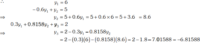
∴ the solution is

3.4.2 Crout’s Method

Consider the system of equations

Now

∴ the system of equations is AX = B

In Crout’s method we factorise A as A = LU, where L is taken as lower triangular matrix and U is taken as unit upper triangular matrix.

That is and

Let UX = Y, so that LY = B, where

Since L and B are known, Y is known.

Substituting Y in UX = Y, we can find X, since U is known.

Thus, we can find the solution of the given system of equations.

Note:

In Crout’s method to find and , we equate the corresponding elements of the columns of A and LU respectively.

That is to find the elements of L and U, we equate the corresponding elements of columns of A and LU.

WORKED EXAMPLES

Example 1

Factorise by Crout’s method.

Solution

Given

By Crout’s method, we take A = LU,

Equating elements of I Columns, we get

Equating elements of II Column, we get

Equating elements of III column, we get

∴

∴

Example 2

Solve the system of equations using Crout’s method.

Solution

The given system of equations is

Here

∴ the given system is AX = B.

By Crout’s method, we take A = LU,

Equating the corresponding elements of I column, we get

Equating the corresponding elements of II columns, we get

Equating the corresponding elements of third column, we get

Put Y = UX, where

∴ LY = B

∴

and

∴ the solution is

Example 3

Solve by Crout’s method, the system of equations .

Solution

The given system of equations is

Here

∴ the given system is AX = B

By Crout’s method, we take A = LU

Equating the corresponding elements of the first columns, we get

Equating the corresponding elements of the second columns, we get

Equating the corresponding elements of third columns, we get

∴

∴

Now

Put UX = Y, where ∴ LY = B

Now

∴ the solution is

3.4.3 Cholesky Decomposition

We have seen the triangular factorisation of a square matrix by Doolittle’s method and Crout’s method. Cholesky decomposition is slightly different from the two methods.

Cholesky method is commonly used in signal processing.

In Cholesky method, to factorise the square matrix, the matrix should be symmetric and positive definite.

A symmetric matrix is positive definite if all the principal minors are positive.

That is if

The principal minors are

and

Definition: Let A be a symmetric matrix and positive definite. Then A can be decomposed as A = LL^T, where L is a lower triangular matrix with digonal elements positive.

L and L^T are called cholesky factors of A.

Application of Cholesky decomposition to solve the system of linear equations

Consider the system of equations

Let

∴ the system of equations is AX = B.

By Cholesky decomposition, let A = LL^T

where

Put where

Since L and B are known, Y is known.

gives X.

WORKED EXAMPLES

Example 1

Obtain Cholesky factorisation of the matrix .

Solution

Let

The elements equidistant from the main diagonal are the same and hence A is symmetrix,

The principal minors are

All the principal minors are positive and so A is positive definite.

So, we can use cholesky method to factorize A. We take A = LL^T

where

and

∴

Equating the corresponding elements of I columns, we get

Equating the corresponding elements of second columns

⇒

Equating the corresponding elements of third columns, we get

⇒

∴

∴

Example 2

Find Cholesky’s factorisation to the matrix . Hence solve the equations .

Solution

Let

A is symmetric and principal minors are

and

∴ A is symmetric and positive definite:

So, we use cholesky’s method to factorize A. We take A = LL^T,

where

∴

Equating the corresponding elements of first columns, we get

Equating the corresponding elements of second columns, we get

and

⇒

Equating the corresponding elements of third columns, we get

∴

The given system of equations is

The coefficient matrix is

This is same as the given matrix A.

∴ the given system of equations is AX = B, where

∴

Put where

⇒ ∴

⇒

⇒

and = 6

⇒

⇒

∴

∴

⇒

⇒

⇒

∴

∴ the solution is

Example 3

Obtain the Cholesky decomposition of and hence solve the system.

AX = b where and .

Solution

Given and it is symmetric

The principal minors are

∴ A is symmetric and positive definite.

So, we can use Cholesky’s decomposition to factorize A. We take A = LL^T

where

∴

Equating Corresponding elements of first columns, we get

Equating corresponding elements of second columns, we get

⇒

⇒

Equating the corresponding elements of third columns, we get

∴

Given AX = b, where and

Now

Put , where ∴

⇒

⇒

∴

and

⇒

∴

Now

⇒

⇒

∴

∴

and

∴

∴ the solution is

Note: In L, if the diagonal elements are not unity, then also we can factorize the given matrix A.

Example 4

Let , then find two triangular matrices L (lower triangular) and U (upper triangular) such that A = LU , using the diagonal elements of L as 3, 1, 5. Hence find A –1.

Solution

Given

Let A = LU, where and

Equating the corresponding elements of each row, we get

∴

Since then where

∴

Exercises 3.5

1. Determine the LU factorisation of the matrix by Doolittle’s method.
2. Determine the LU factorisation of the matrix by Doolittle’s method.

   (I) Solve by using Doolittle’s method the following system equations.

3. 
4. 
5. 
6. 
7. Find the LU factorisation of the matrix by Doolittle’s method and hence solve the system of equations .
8. Given , find the LU factorisation of A by Doolittle’s method and hence solve the system of equations AX = B where .

   (II) Solve by using Crout’s method the following system of equations.

9. 
10. 
11. 
12. Find the inverse of using crout’s method.
13. Find the crout’s factorisation of the matrix .

    (III) Solve by using Cholesky’s method

14. 
15. 
16. 
17. Find the Cholesky decomposition of the matrix A = and hence solve the system AX = B, where and .
18. Find the Cholesky factorisation of the matrix and hence solve the system AX = B, where and .
19. Find the Cholesky decomposition for the matrix .

Answers 3.5

1. and
2. and
3. (4)
4. (6)
5. 
6. 
7. (10)
8. 
9. 
10. (14)
11. (16)
12. 
13. 
14. 

Short Answer Questions

1. What are direct methods?
2. What are indirect methods?
3. Give two direct methods to solve a system of linear equations.
4. Give two indirect methods to solve a system of linear equations.
5. Using Gauss elimination method solve .
6. Explain briefly Gauss-Seidel method of solving simultaneous linear equations.
7. Solve the linear system by Gauss-Jordan method.
8. What is the condition for convergence of Gauss-Seidel method?
9. Why Gauss-Seidel methd is better than Jacobi’s-iterative method?
10. Compare Gauss elimination and Gauss-Seidel method?
11. If we start with zero values for x, y, z while solving by Gauss-Seidel iteration, find the values for x, y, z after one iteration.
12. Find the inverse of by Gauss-Jordan method.
13. Find the first iteration values of x, y, z satisfying by Gauss-Seidel method.
14. Given find the inverse of the coefficient matrix.
15. Solve by Jordan’s method.
16. Write down the sufficient conditions for the solution of the linear system Ax = B by LU method of Doolittle or Crout.
17. Write down the sufficient Condition for the solution of the linear system Ax = B by Cholesky’s method.
18. Factorize by Doolittle’s method.
19. Factorize by Crout’s method.
20. Factorize by Choleskey’s method.
21. What is the drawback of Jacobi’s method in finding the eigen values of a symmetric matrix?
22. What is the minimum number of rotations required to bring the symmetric matrix A of order n in to diagonal form.
23. Determine the largest eigen value and the corresponding eigen vector of the matrix correct to two decimal places using power method.
24. Write down all possible types of initial vectors to determine the largest eigen value and the corresponding eigen vector of a matrix of size .