8.0 INTRODUCTION

Quite often in engineering and science, we conduct experiments involving two quantities, say x and y. Suppose x₁, x₂, ...,x_n be the values of x corresponding to which the values of y are y₁, y₂ ..., y_n. We would like to know the functional relation between x and y. As a first step we plot the points (x₁, y₁), (x₂, y₂), .... (x_n, y_n) with respect to rectangular axes. The resulting set of points plotted is called a scatter diagram. From the scatter diagram it is possible to visualize a smooth curve which passes as closely as possible to these points and that approximates the data. Such a curve is called an approximating curve.

The equation of this curve between x and y is called an empirical relation.

For example, in the scatter diagram if the points cluster around a straight line, then we say that a linear relationship exists between x and y. If the points cluster around a curve, then we say a non–linear relationship exists between x and y.

The general problem of finding the equation of the approximating curve that fits the given set of data is called curve fitting.

If the relation is linear, then we assume the empirical relation of the approximating curve as y = ax + b.

The best values of the constants occurring in the equation can be found in different ways. We shall fit a curve by the following methods:

1. method of least squares
2. method of averages
3. method of the sum of exponentials
4. method of moments

8.1 METHOD OF LEAST SQUARES

Let (x₁, y₁), (x₂, y₂), ..., (xn, yn) be a set of observed data and let y = f (x) be the relation suggested by the scatter diagram.

Let Pi be the point (xi, yi), i = 1,2, 3, ..., n

When x = xi, the observed value is yi and the expected value is f (xi).

Let di = yi – f (xi) be the difference between the observed and expected values for each i.

The differences d₁, d₂, ..., dn are called the residuals, which may be positive or negative

The principle of least squares is that the sum of the squares of the residuals is minimum.

It is also referred as Gauss’s least square principle.

The curve fitted by this principle is called the least square curve.

The curve for which is minimum is called a best fitting curve besides all the curves approximating the given set of points.

A line fitted by this principle is known as least-square line and a parabola fitted by this principle is known as least square parabola.

Note: The method of least squares gives unique values for the constants and so the curve fitted is unique.

8.1.1 Fit a Straight Line by the Method of Least Squares

Let (x₁, y₁), (x₂, y₂) ... (xn, yn) be a set of observed values of the variables x and y.

Let the relation between x and y be y = ax + b(1)

Then, the sum of squares of residuals is

⇒

By principle of least squares E is minimum.

Since xi and yi are known, E is a function of a and b.

The conditions for E to be minimum are and

and

(2)

(3)

Solving (2) and (3), we get the values of a and b.

For these values of a and b, the line y = ax + b is the best fitted line to the data.

The equations (2) and (3) are called the normal equations for the least–squares line

y = ax + b

Note:

1. The formulae can be remembered by omitting the suffixes:

   The line is y = ax + b (1)

   The normal equations are Σy = aΣx + nb

   and Σxy = aΣx² + bΣx

2. If the values of x are equally spaced with interval h, we can simplify the computation by changing the origin and scale by the transformation

   so that

WORKED EXAMPLES

Example 1

Use the method of least squares to fit a straight line to the following data:

x	0	5	10	15	20
y	7	11	16	20	26

Estimate the value of y when x = 25.

Solution

We fit a straight line to the given data by the method of least squares.

Since the values of x are equally spaced, let

Then the equation of the line of best fit is

y = aX + b (1)

Normal equations are (2)

and (3)

To find we form the table

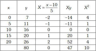
From the table

Substituting in (2), we get 80 = a.0 + 5b ⇒

Substituting in (3), we get 47 = a.10 + b.0 ⇒

⇒ the equation of the line of best fit is

When x = 25, y = 0.94(25) + 6.6 = 30.1

Example 2

In a tensile test of a metal bar the following observation were made where x represents load in tons and y elongation in ten thousands of an inch.

x	1	2	3	4	5	6
y	14	27	41	56	68	75

Using the principle of least squares, find a law of the form y = ax + b.

Solution

We fit a straight line by the principle of least squares.

Here the values of x are equally spaced with h = 1, but n = 6.

So, we choose the origin as the average of the two middle values 3 and 4 and it is

Let X = x – 3.5

Then, the equation of the line of best fit is y = aX + b

The normal equations are (2)

and (3)

Substituting in (2), we get,

Substituting in (3), we get,

⇒ the equations of the line of best fit is

 

Example 3

Using 1964 as the origin obtain a straight line trend equation by the method of least squares.

Year	1960	1962	1963	1964	1965	1966	1969
Value	140	144	160	152	168	176	180

Find the trend value of the missing year 1961.

Solution

Let the year be denoted by x, and let the value be denoted by y

Let

X = x – 1964

Then, the equation of the straight line of best fit is

y = aX + b(1)

the normal equations are (2)

and

(3)

⇒ The normal equations are

1120 = a.1 + 7b

⇒ 1120 = a + 7b (4)

and

412 = a × 51 + b.1

⇒ 412 = 51a + b(5)

(4) – 7 × (5) ⇒ 1120 – 2884 = a (1 – 357)

⇒ 356 a = 1764

⇒ a = = 4.955 = 4.96

Substituting in (4), we get

7b + 4.96 = 1120

⇒ 7b = 1120 – 4.96 = 1115.04

⇒ b =

The straight line trend is y = 4.96X + 159.29

⇒ y = 4.96(x – 1964) + 159.24

When x = 1961,

y = 4.96 (1961 – 1964) + 159.29

⇒ y = 4.96(–3) + 159.29

⇒ y = –14.88 + 159.29 = 144.41

∴ the trend value for the year 1961 is 144.41.

8.1.1 (a) Fitting Other Type of Equations Reducible to the Form

Certain types of equations can be reduced to the linear form by transformation of variables.

This process is usually called rectification.

Some of such equations are given below.

WORKED EXAMPLES

Example 4

An experiment on the life of a cutting tool at different cutting speeds gave the values given below.

Speed vft/min	350	400	500	600
Life Tin min.	61	26	7	2.6

It is known that v and T satisfy the relationship v = aT b. Using the method of least squares find the best values of a and b.

Solution

Given v = a Tb

Taking log to the base 10

log₁₀ v = log₁₀ a + b log₁₀ T

Put Y = log₁₀ v, A = log₁₀ a, X = log₁₀ T

Then, the equation is Y = A + bX (1)

which is linear in x and y.

The normal equations are

(2)

(3)

We form the table

Substituting in (2) and (3), we get

Example 5

The voltage v across a capacitor at time t seconds is given by the following table. Use the principle of least squares to fit a curve of the form v = aekt to the data.

t	0	2	4	6	8
v	150	63	28	12	5.6

Solution

Given v= aekt.

Taking log to base 10, we get

log_l0v= log₁₀ a + kt log₁₀ e

Put Y= log₁₀ v, A = log₁₀ a, B = klog₁₀e,

∴ the equation is Y= A + BX (1)

By method of least squares, the normal equations are

(2)

and

(3)

We form the table

Substituting in (1), we get 7.2499 = 5A + B.0

Substituting in (3), we get

–3.5759 = A.0 + B.10

A = 1.45 ⇒ log₁₀ a = 1.45 ⇒ a = 10^1.45 = 28.184

B = –0.3576

⇒ k log₁₀ e = –0.3576

= −0.3576 log_e10

= −0.3576(2.30258) = −0.8234

∴ v = 28.184 e^–0.8234t

8.1.1 (b) Fit a Parabola y = ax2 + bx + c by the Method of Least Squares

Let (), (), … () be n observed values of x and y.

We have to fit the parabola y = ax² + bx + c (1)

to this data

The sum of the squares of the residuals is

Since xi and yi. are known, E is a function of a, b, c.

By principle of least squares E is minimum.

the conditions are

(2)

Similarly, (3)

and (4)

Solving (2), (3) and (4) we get the values of a, b, c for which the curve y = ax² + bx + c is the best fitted curve to the data.

Note: Dropping the suffixes, for simplicity, the normal equations of the least square curve

y = ax² + bx + c(1)

are Σy = aΣx² + bΣx + nc(2)

Σxy = aΣx³ + bΣx² + cΣx(3)

Σx²y = aΣx⁴ + bΣx³ + cΣx²(4)

They can be remembered as below

Taking Σ of (1) we get (2)

Multiply (1) by x and then taking Σ, we get (3)

Multiplying (1) by x² and then taking Σ, we get (4).

WORKED EXAMPLES

Example 1

Fit a parabola of the form y = ax2 + bx + c to the following data:

x	0	1	2	3	4
y	1	1.8	1.3	2.5	6.3

Solution

We fit a parabola to the given data by the method of least square.

The values of x are equally spaced with h = 1

For simplicity in computation we take origin for x.

Put

X = x − 2.

Then the equation of the curve of best fit is

y = aX² + bX + c (1)

The normal equations are

(2)

(3)

(4)

We form the table

Substituting in (2), we get 12.9 = 10a + b.0+5c

10a + 5c = 12.9

2a + c = 2.58 (5)

Substituting in (3), 11.3 = a.0 + b(10) + c.0

10 b = 11.3 b = 1.13

Substituting in (4), 33.5 = a.34 + b.0 + c.10

34a + 10c = 33.5

Dividing by 10, 3.4a + c = 3.35 (6)

(6) – (5) 1.4a = 0.77

Substituting in (5), we get c = 2.58 − 2(0.55) = 2.58 – 1.10 = 1.48

The curve of best fit is y = 0.55X² + 1.13X + 1.48, where X = x – 2

Example 2

The following table gives the levels of prices in certain years. Fit a second degree parabola to the data:

Year	1975	1976	1977	1978	1979	1980	1981	1982	1983	1984	1985
Price	88	87	81	78	74	79	85	84	90	92	100

Solution

We fit a parabola, to the given data by the method of least squares.

Let x denote year and y denote price.

For year, take the origin as 1980. Let X = x – 1980.

Then the equation of the best fitted curve is

y = aX² + bX + c (1)

The normal equations are

(2)

(3)

(4)

we form the table

n = 11, y = 938, X = 0, X² = 110, X³ = 0, X⁴ = 1958, Xy = 130, X²y = 9910

Substituting in (3) we get, 130 = a.0 + b.110 + c.0

Substituting in (2), we get 938 = a × 110 + b.0 + 11 × c

110a + 11c = 938

10a + c = 85.2727(5)

Substituting in (4), 9910 = 1958a + 0.b + 110c

1958a + 110 c = 9910

Dividing by 110, 17.8a + c = 90.0909(6)

(6) – (5) 7.8a = 4.8182

Thus a = 0.62, b = 1.18, c = 79.10

The curve of best fit is where X = x – 1880

Example 3

Fit a second degree parabola of the form y = ax²+ bx+ cto the following data taking xas the independent variable.

x	1	2	3	4	5	6	7	8	9
y	2	6	7	8	10	11	11	10	9

and introducing the new variable uand vby the equations u = x - 5, v = y - 7.

Solution

We fit a parabola to the given data by the method of least squares.

Since the given new variables are u and v and u = x – 5,v = y – 7, taking u as the independent variable, and v as the dependent variable the equation of the parabola in u and v is

v = au² + bu + c (1)

The normal equations are

(2)

n = 9, u = 0, u² = 60, u³ = 0,

u⁴ = 708, v = 11, uv = 51, u²v = −9

Substituting in (2), (3) and (4), we get

11 = a × 60 + b × 0 + 9c

60a + 9c = 11

6.6667a + c = 1.2222 (5)

51 = a.0 + b.60 + c.0

60b = 51 b = = 0.85 (6)

and – 9 = a × 708 + b.0 + c × 60

708a + 60c = − 9

a + c =

11.8a + c = 0.15 (7)

(7) − (5) 5.1333a = 1.3722

(5) c = 1.2222 − 6.6667 × (–0.2673)

= 1.222 + 1.7820 = 3.0042

a = −0.2673, b = 0.85, c = 3.0042

v = –0.2673 u² + 0.85u + 3.0042

y – 7 = −0.2673 (x – 5)² + 0.85 (x – 5 ) + 3.0042

y = 7 – 0.2673 (x² – 10x + 25) + 0.85x – 4.25) + 3.0042

y = – 0.2673x² + 3.523x – 0.9283

Example 4

Fit a parabola of the form y = ax²+ bx+ cto the following data by the method of least squares and predict the value of ywhen x = 70.

X	71	68	73	69	67	65	66	67
Y	69	72	70	70	68	67	68	64

Solution

We have to fit a parabola of the form y = ax² + bx + c by the method of least squares.

Let X = x – 67, Y = y –70

the equation is Y = aX² + bX + c (1)

The normal equations are

we form the table

n = 10, X = 10, , X³ = 280,

X⁴ = 1586, XY = 6, X²Y = –28

Substituting in (2), (3) and (4), we get

–12 = a × b2 + b × 10 + 8c

7.75a + 1.25b + c = –1.5(5) [Dividing by 8]

6 = a × 280 + b × 62 + c × 10

28a + 6.2b + c = 0.6 (6) [Dividing by 10]

and –28 = a × 1586 + b × 280 + c × 62

25.58a + 4.52b + c = –0.45 (7) [Dividing by 62]

(6) − (5) 20.25a + 4.5b = 2.1

4.09 a + b = 0.4242 (8)

(6) – (7) 2.42a + 1.68b = 0.15

1.44 a + b = 0.089 (9)

(8) – (9) 2.65a = 0.3352

(9) b = 0.089 – 1.44 × 0.1265

= 0.089 – 0.182 = –0.093

c = 0.6 – 28 × 0.1265 – 6.2 (–0.093)

= 0.6 – 3.542 + 0.5766 = –2.3654

∴ The equation of the parabola is

Y = 0.1265 X² – 0.093X – 2.3654

y – 70 = 0.1265 (x – 67 )² − 0.093(x – 67) – 2.3654

y = 0.1265x² – (0.093 + 16.95)x

+ 567.8585 + 6.231 – 2.3654 + 70

y = 0.1265x² – 17.043 x + 641.724

When x = 70, y = 0.1265 × 70² – 17.043 × 70 + 641.724

y = 619.85 – 1193.01 + 641.724 = 68.564 = 69

Exercises 8.1

By method of least squares fit the indicated curve to the given data:

Fit a straight line to the data:

x	0	1	2	3	4
y	1	1.8	3.3	4.5	6.3

Fit a straight line to the data:

x	75	80	93	65	87	71	98	68	84	77
y	82	78	86	72	91	80	95	72	89	74

(3) Find the least square line for the data below:

x	1	2	4	6	8	9	11	14
y	1	2	4	4	5	7	8	9

smoothen the data in the above by using the least square line.

(4) The weights of calf taken at weekly intervals are supplied below. Fit a straight line and calculate the average rate of growth per week.

Age x	1	2	3	4	5	6	7	8	9	10
Weight y	52.5	58.7	65.0	70.2	75.4	81.1	87.2	95.5	102.2	106.4

(5) Fit a curve of the form y = ax + bx² to the data:

x	1	2	3	4	5
y	1.8	5.1	8.9	14.1	19.8

Calculate y when x = 2.

(6) Given

x	2	4	6	8
y	5.5	14.5	26.2	41.8

Fit a law of the form y = ax + bx² by computing the least square line.

(7) For the law of the + bx, find the best values of a and b from the following data

x	1	2	3	4	5	6
y	5.4	6.3	8.2	10.2	12.6	15

(8) Fit an equation of the form y = ae^bx for the data

x	1	2	3	4
y	1.65	2.70	4.50	7.35

(9) The pressure and volume of a gas are known to be related by the equation pv = c, a constant. In an experiment, the following volumes of quantity of gas were observed for the pressures specified. Fit the same equation taking P as independent variable.

P (kg/sq.cm)	0.5	1.0	1.5	2.0	2.5	3.0
v (litres)	1.62	1.00	0.75	0.62	0.52	0.46

Growth of bacteria (y) in a culture after x hours is given in the following table. Fit a curve of the form y = abx by method of least squares.

House x	0	1	2	3	4	5	6
No. of bacteria y	32	47	65	92	132	190	275

Estimate y when x = 7.

Find the least squares parabola for the data:

x	0	2	4	6	8	10
y	1	3	13	31	57	91

Find the least square parabola to the data:

x	0	1	2	3	4
y	1	5	10	22	38

Answers 8.1

(1) y = 1.33x + 0.72, (2) y = 0.66x + 29.13

(3) The least square line is y = 0.62x + 0.75

The estimated values of y obtained from this line corresponding to x = 1,2, … 9,11,14 are the smoothening values. The smoothened values of y are 1.37, 1.99, 3.23, 4.47, 5.71, 633, 7.57, 9.43

(4) y = 6.16 x + 45.74, rate of growth = 6.16 (5) When x = 2, y = 486

(6) Y = 1.95 + 0.41x and y = 1.95x + 0.41x² (7) a = 2.7907, b = 2.413

(8) y = e^0.4994x (9) Pv^0.422 = 0.9972

(10) y = 32.15 (1.427)x ; when x = 7, y = 387 (11) y = x² – x + 1

(12) y = 2.2x² + 0.3x + 1.4

8.2 METHOD OF GROUP AVERAGES

Let (x₁, y₁). (x₂, y₂), (x₃, y₃), … (xn,yn) be the set of observed values of the related variables x and y.

Let y = a + bx (1)

be the assumed linear relationship between the two variables.

To determine the constants a and b, we need two equations in a and b.

When x = x₁, the observed value of y is y₁ and the estimated values of y from (1) is a + bx₁

Their difference is called residual or deviation.

Thus d₁= y₁– (a + bx₁) is the residual for the point (x₁, y₁).

Similarly for the other points we find the residuals

d₂ = y₂ – (a + bx₂), d₃ = y₃ – (a + bx₃), … d_n = y_n – (a + bx_n)

Some of the residuals may be positive, some of them may be negative or zero. The method of group averages is based on the assumption that the sum of the residuals is zero. ie.

Since we require two equations in a and b to find out the values of a and b, we divide the given data into two groups such that the sum of residuals is zero for each group.

Let the first group contain r observations, say, (x₁, y₁), (x₂, y₂), (x₃, y₃), … (x_r,y_r) and the second group contain remaining (n – r) observations.

Dividing by r, we get

(2)

where

Similarly

Dividing by (n – r),

where

Solving (2) and (3), we get a and b.

Substituting the values of a and b in (1), we get the line fitted to the data.

Note:

• (1) Since and are the average values of x and y in the first group and , are the average values of x and y in the second group, the method is known as method of averages.
• If we divide the data into two groups in a different way such that the sum of the residuals is zero in each group, then the values of a and b will be different, and so the equation will be different. This is the serious draw back of this method.
• Since y = a + bx is satisfied by () and (), this line is the line joining the points () and (). So the equation of the line fitted to the data is
• (4) In practice, we divide the data into two groups which contain the same number of points.

WORKED EXAMPLES

Example 1

Fit a straight line of the form y = a + bx by the method of group averages for the following data:

x	0	5	10	15	20	25
y	12	15	17	22	24	30

Solution

Given 6 sets of values, we divide it into two groups each containing 3 sets of values.

∴

∴ the equation of the line fitted to the data is

Example 2

The weights of a calf taken at weekly intervals are given below. Fit a straight line by method of averages.

Age in weeks	1	2	3	4	5	6	7	8	9	10
Weight	52.5	58.7	65	70.2	75.4	81.1	87.2	95.5	102.2	108.4

Calculate also the average rate of growth per week.

Solution

Let x denote the age in weeks and y denote the corresponding weight.

We divide the given data of 10 values into two groups of 5 values each.

Equation of the straight line fitted to data is

The rate of growth is

Example 3

Experimental values of two connected quantities x, yare given below:

x	1	2	3	4	5	6
y	2.6	5.4	8.7	12.1	16	20.2

If the relation between x and y is y = ax + bx² where a and b are constants, find the best values of a and b.

Solution

The given equation is y = ax + bx²

⇒ y = x (a + bx)

⇒

Put and X = x. Then the equation is Y = a + bX, which is linear in X and Y.

Divide the given set of 6 values into two groups of 3 values each.

∴ the linear equation in X and Y is

⇒

Example 4

The data in the following table fit a formula of the type y = axn. Find the values of aand nand the formula by the method of group averages.

x	10	20	30	40	50	60	70	80
y	1.06	1.33	1.52	1.68	1.81	1.91	2.01	2.11

Solution

Given y = axn

Taking log to the base 10,

log₁₀ y = log₁₀ a + n log₁₀ x

Put Y = log₁₀ y, X = log₁₀ x and A = log₁₀ a

∴ the equation is Y = A + nX, which is linear in X and Y.

Divide the given data into two groups of 4 values each.

∴ the equation in X and Y is

Example 5

Fit a curve of the form to the following data by the method of averages.

x	8	10	15	20	30	40
y	13	14	15.4	16.3	17.2	17.8

Hence find the values of a and b.

Solution

Given

Put

∴ the equation is Y = aX + b, which is linear in x and y.

Divide the given data into two groups of 3 values each.

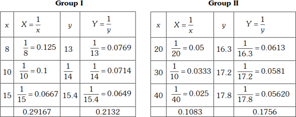
∴the equation in X and Y is

Type 2. Equations of the form y = a + bx + cx²

We reduce this equation to the above type and solve.

Let (x₁,y₁) be a particular point on y = a + bx + cx² satisfying the equation.

Then, y₁ = a + bx₁ + cx₁²

Then, we get Y = b + cX, which is linear in X and Y.

We use group average method to find b and c.

Example 6

The data given below will fit a formula of the type y = a + bx + cx2. Find the formula.

x	87.5	84.0	77.8	63.7	46.7	36.9
y	292	283	270	235	197	181

Solution

Given y = a + bx + cx²(1)

Taking (87.5, 292) as a particular point on (1), we get

292 = a + b(87.5) + c(87.5)²(2)

(1) − (2)⇒ y – 292 = b[x – 87.5] + c[x² – (87.5)²]

= (x – 87.5) [b + c(x + 87.5)]

⇒

To find b and c, we use the group average method.

Divide the given data into two groups of 3 values each.

∴ the equation in X and Y is

⇒

⇒

⇒

= 0.00358(X−168.4)

= 0.00358X−0.6029

⇒ Y = 0.00358X+2.4197−0.6029

⇒ Y = 0.00358X+1.8168

Exercises 8.2

By the method of group averages fit the indicated curve.

(1) Fit y = ax + b to the data

x	50	70	100	120
y	12	15	21	25

(2) The following numbers relate to the flow of water over a triangular notch:

H	1.2	1.4	1.6	1.8	2.0	2.4
Q	4.2	6.1	8.5	11.5	14.9	23.5

H denotes the head of water (in feet), Q the quantity (in cubic feet) of water flowing per second. If the law is Q = CHn, find the best values of C and n.

[Hint: log₁₀Q = log₁₀C + nlog₁₀H; put Y = log₁₀Q, A = log₁₀C, X = log₁₀H

⇒ Y = A + nX]

(3) Fit a curve of the form y = kxn given:

x	25.9	259	2590	25900
y	0.308	0.209	0.148	0.098

(4) Fit a curve of the form y = a + bx + cx² for the data:

x	2	2.5	3	3.5	4	4.5	5	5.5	6
y	18	17.8	17.5	17	15.8	14.8	13.3	11.7	9

Answers 8.2

(1) y = 0.19x + 2.1 (2) C = 2.6, n = 2.5

(3) y = 0.2673x−^0.0118 (4) y = 15.8 + 2.1x − 0.5x²

8.3 METHOD OF THE SUM OF EXPONENTIALS

We shall now discuss another type of curve fitting known as exponential curve fitting.

Let be the observed data for the variables x and y.

Let

(1)

be the curve fitted to the data, where are constants to be determined. We shall assume n is fixed and is known.

We know that is the solution of the differential equation of the form

(2)

where are unknown constants and are the roots of the auxiliary equation

(3)

By Froberg’s method (1965), we can compute the derivatives numerically at the n points and substitute in (2) which will result in a system of n linear equations in the n unknowns which can be solved. Then can be obtained and finally can be obtained from (1) by the method of least squares or the method of averages.

Thus is fitted to the given data

Note: The drawback of this method is the unreliability of the results, because of the accuracy of the derivatives decreases as the order n increases.

We shall now discuss a method given by Moore in 1974 which gives more reliable results. For simplicity, we shall consider the case when .

Let the curve to be fitted to the data be

(4)

This function is the solution of the second order differential equation

(5)

where are constants to be determined and are the roots of the auxiliary equation

.

Let ‘a’ be the initial value of x.

Integrating (5) w.r.to x, we get

where

Again integrating w.r.to x, we get

⇒

We know the formula

(6)

Let and be two data points such that , then

(7)

and (8)

Taking two different and evaluating these integrals by numerical method, say Simpson’s rule, we get two linear equations in and .

Solving these equations, we get and .

Solving , we get the values of and .

Finally, we find the values of and by the method of least squares or averaging method.

Thus is fitted to the data.

WORKED EXAMPLES

Example 1

Fit a function of the form to the following data.

x	1	1.1	1.2	1.3	1.4	1.5	1.6	1.7	1.8
y	1.175	1.336	1.510	1.698	1.904	2.129	2.376	2.646	2.942

Solution

The curve fitted to the given data is the solution of the differential equation

The auxiliary equation is

(1)

Let be the roots of the auxiliary equation.

The coefficients are given by

(2)

where a is the initial value of x and x₁ and x₂ are two data points such that

To evaluate the integrals, we use Simpson’s rule.

So, we choose such that there are even number of intervals.

⇒ choose

⇒

Substituting in (2), we get

The given table is

We shall evaluate these integrals by Simpson’s rule

Now take and . We get

We shall evaluate these integrals by Simpson’s rule.

Substituting in (1), we get

We take and

∴

To find and , we use the method of least squares

The sum of the squares of the residuals is

According to the method of least squares E is minimum if and

(5)

(6)

The equations (5) and (6) are called the normal equations.

Now we shall form the table for computation

Substituting in (5) and (6), we get

Dividing by 7.8267, we get

(7)

and

Dividing by 0.4838, we get,

(8)

Substituting in (7), we get

∴

which is the equation of the curve fitted to the given data.

Example 2

Fit a curve of the form whose equation is , using the following data.

x	1	1.1	1.2	1.3	1.4	1.5	1.6	1.7	1.8
y	1.54	1.67	1.81	1.97	2.15	2.35	2.58	2.83	3.11

Solution

The curve given by y = A₁e^λ₁^x + A₂e^λ₂^x fitted to the data is the solution of the differential equation

The auxiliary equation is

λ² = a₁λ + a₂(1)

Let λ₁, λ₂ be the root of the auxiliary equation

The co-efficients a₁, a₂ are given by

Where a is the value of x and x₁, x₂ are two data points such that

To evaluate the integrals, we use Simpson’s rule.

So, we choose in such way that there are even number of intervals between and and the last value of x

choose and

Substituting in (2), we get

The given data is

x	1	1.1	1.2	1.3	1.4	1.5	1.6	1.7	1.8
y	1.54	1.67	1.81	1.97	2.15	2.35	2.58	2.83	3.11

We shall evaluate these integrals by Simpson’s rule.

∴

⇒

Dividing by 0.0604, we get

Now take and

⇒

Substituting in (2), we get

We shall evaluate these integrals by Simpson’s rule

Dividing by 0.096, we get

(4)

Substituting in (4), we get

⇒

Substituting in (1), we get

We take and

⇒

We shall now find , by the method of least squares.

The sum of the squares of the residuals is

According to the method of least squares E is minimum for the best fitted curve.

The normal equations are given by and .

(5)

(6)

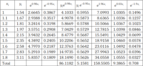
Substituting in the normal equations (5) and (6), we get

Dividing by 9.3685, we get

(7)

and

Dividing by 0.708, we get

(8)

Substituting in (8), we get

Take A₁ = 0.52, and A₂ = 0.39

∴

Which is the equation of the curve fitted to the given data.

Exercise 8.3

(1) Fit a curve of the form for the following data

x	2	2.2	2.4	2.6	2.8	3.0	3.2	3.4	3.6
y	3.63	4.46	5.47	6.70	8.19	10.02	12.25	14.97	18.29

Answer 8.3

(1)

8.4 METHOD OF MOMENTS

Let (x₁, y₁), (x₂, y₂), … (xn, yn) be a set of n observations of the related variables x and y.

Let the values of x be equally spaced with interval h = Δx, say

ie. xi− xi = Δx for all i = 1, 2, 3, ..., n − 1.

For such a set of points, we define

the first moment μ₁ = Σy Δx = Δx Σy

the second moment μ₂ = Σ xy Δx = Δx Σ xy

the third moment μ₃ = Σ x²y Δx = Δx Σx²y and so on.

These moments are called the moments of the observed values of y.

Let y = f(x)be the curve to be fitted the data.

Then, the first moment g₁ = ∫y dx = ∫f(x) dx

the second moment g₂ = ∫xy dx = ∫xf(x) dx

and the third moment g₃ = ∫x²y dx = ∫x² f(x) dx and so on.

These moments are called the moments of the computed values of y or expected values of y.

The method of moments is based on the assumption that the moments of the observed values of y is equal to the moments of the expected values of y.

i.e. mI = ri

It can be proved that

These equations are known as observation equations.

If the form of f(x) is known, then using the observation equations the constants can be determined.

If f(x) is linear ie. f(x) = ax + b, then the equation of the curve fitted is y = ax + b

If

Solving these two equations we find a and b and hence the equation y = ax+b

WORKED EXAMPLES

Example 1

By the method of moments, obtain a straight line to fit the data.

x	1	2	3	4
y	0.30	0.64	1.32	5.40

Solution

We fit a straight line to the given data by the method of moments.

Given values of x are equally spaced with Δx = 1.

Here x₁ = 1, xn = 4

⇒

Let the line fitted be y = ax+b (1)

Then, the observation equations are

Now

and

Substituting in (2) and (3) we get

(4)

and

30.333a + 10b = 27.14

Dividing by 10, 3.0333a + b = 2.714(5)

(5) − (4) ⇒

∴ b = 1.915 − 2.5(1.499) = −1.8325

∴ the equation of the straight line is y = 1.499x - 1.8325

Example 2

By method of moments fit a straight line to the data:

x	1	2	3	4
y	0.17	0.18	0.23	0.32

Solution

We fit a straight line to the given data by the method of moments.

Given values of x are equally spaced with

∴

Let the line fitted be y = (1)

Then, the observation equations are

(2)

(3)

Now

Substituting in (2),

(4)

Substituting in (3),

(5)

Exercises 8.4

Fit a straight line by the method of moments to the following data:

x	1	2	3	4
y	16	19	23	26

Fit a straight line by the method of moments to the following data:

x	1	3	5	7	9
y	1.5	2.8	4.0	4.7	6.0

Fit a straight line by the method of moments to the following data:

x	1	2	3	4
y	1.7	1.8	2.3	3.2

Fit a straight line by the method of moments to the following data:

x	0	1	2	3	4	5
y	66.7	72.7	82.3	92.1	93	100

Answers 8.4

(1) y = 3.188x + 13.03 (2) y = 0.5231x + 1.1845

(3) y = 0.49x + 1.025 (4) y = 6.86x + 67.4

SHORT ANSWER QUESTIONS

1. What is meant by curve fitting?

2. State the principle of least square.

3. Define residual.

4. Write the normal equations to fit a straight line of the form

5. Write down the normal equations to fit a quadratic curve by the method of least squares.

6. Define the method of group averages.

7. Convert the equation into a linear form where a and b are constants.

8. Convert

9. Convert the equation into linear form.

10. Convert into linear form.

11. What is Gauss’s least square principal.

12. Convert into linear form.

13. Explain method of group Averages.

14. What is the defect of method of group averages?

15. How to avoid the defect of method of group averages?

16. is fitted by the method of moments.

17. Convert into linear form.

18. Convert into linear form.

19. Convert into linear form.

to a linear form and write the corresponding normal equations to fit it.