9.0 INTRODUCTION

Many problems in science and engineering can be reduced to the problem of solving differential equations satisfying certain conditions. For example, spring-mass systems, resistor- capacitor-inductance circuits, bending of beams, chemical reactions, pendulums, simple harmonic motions, the motion of a rotating mass and so on. Using analytical methods we can solve only standard types of differential equations. But the differential equations appearing in practical problems of engineering and science are not of the standard types and are complex. So, it is rather impossible to find closed form solutions. Such equations are solved by numerical methods where the solution is given as a table of values of the function at various values of the independent variable. This is called point wise solution. Such methods are called pointwise methods or single step methods because they use at to find at . In contrast we have methods like Milne’s and Adam’s which use to find . So they are called multistep methods.

We shall consider some of the methods commonly used to solve differential equations.

9.1 TAYLOR’S SERIES METHOD

Consider the first order differential equation with initial condition .

We can expand as a power series in in the neighbourhood of by Taylor’s series.

∴

Put

∴

If , then

Now y can be expanded as Taylor’s series about and we have

Continuing this way, we find

where

The solution y (x) is given as a sequence

1. If we calculate the value of by omitting and higher powers of h, the truncation error will be where k is a constant and the corresponding Taylor’s series is said to be of second order.

   If h is small and terms after n terms are neglected the error is where if

2. It is a single step method. If f(x, y) is complicated function, higher derivatives cannot be found and so the method can not be used. This is the draw back of the method.

WORKED EXAMPLES

Example 1

Solve by Taylor’s series method. Find the values of y at x = 0.1 and x = 0.2.

Solution

Given

∴

Taylor’s series is (1)

We have

Differentiating we get,

At (x0, y0) = (0,1),

Substituting r = 0 in (1), we get

Now

Put in (1), we get

At (x1, y1) = (0.1, 1.1103),

∴

the solution is

Example 2

Using Taylor’s series method find y at x = 0, if .

Solution

Given

Taylor’s series is (1)

and y ′″ = x²y ″+ 2xy ′ + 2(xy ′+ y.1)

At y ′0 = 0 - 1 = -1

y ″0 = 0 + 0 = 0

y ′″0 = 0 + 0 + 0 + 2.1 = 2

Putting in (1), we get

Example 3

Using Taylor’s series method find y(1.1) and y(1.2) correct to four places given and

Solution

Given

Required

Taylor’s series is (1)

we have

and

At

Putting in (1), we get

Now

Putting ,we get

At

∴

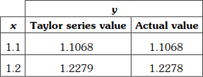
Thus

Since this equation is a simple variable separable equation we can solve and find the exact solution. We shall compare the computed value with the exact value.

where

So, solution is

When = 1.1068

When = 1.2278

Example 4

Using Taylor’s series method find y at x = 1.1 and 1.2 by solving , given

Solution

Given

Required y at

Taylor’s series is

(1)

we have

∴

and

At

Putting in (1), we get,

∴

∴

Now

Putting in (1), we get,

At

∴

∴

Hence

Example 5

Use Taylor series method to find given that correct to 4 decimal accuracy.

Solution

Given equation is and y(0) = 0

∴

Required ∴ h = 0.1

Taylor’s series is (1)

We have

∴

and

Putting in (1), we get,

At

∴

∴

Now

Putting in (1), we get

At

∴

∴ y (0.2) = 0.8108

∴

9.2 EULER’S METHOD AND MODIFIED EULER’S METHOD

Euler’s method is one of the simplest and oldest methods of finding numerical solution of differential equation. It is a step-by-step method because the values of y are computed by short steps ahead for equal intervals of the independent variable. This crude method is rarely used in practice but it explains the principle of methods based on Taylor’s series.

Consider the differential equation

Let be equidistant values of x where

so that

In Euler’s method we approximate a curve in a small interval by a straight line.

Let be the curve representing the actual solution.

Equation of the tangent at is

∴

Since the curve in the interval is approximated by this straight line, the value of y at is approximately

Similarly the curve in the interval is approximated by the line through and having slope

∴

Proceeding in this way we get the general formula

This is called Euler’s algorithm:

Note:

1. Since and , the above formula can be simply written as
2. The draw back of this method is that it is either too slow (in case h is small) or too inaccurate (in case h is not small).
3. The computed y’s will deviate more and more from the true y’s as we proceed further along X-axis, due to cumulative rounding errors.

These drawbacks have led to a modification of Euler’s method aiming at more accurate results.

We start with the tangent at .

Let the ordinate at intersect the tangent at Q, where

We find the slope at Q.

ie

We draw the line through Q with this as slope and let this line be .

We then draw the line L through parallel to .

This line L is taken as an approximation to the curve in the interval .

Equation of L is

When

ie.

Proceeding this way, in general we have

where

Note:

(1) The above formula is one version of the modified formula. It gives a better approximation. In this method we took average of points.

(2) Another version of Euler modified formula is given in terms of the average of the slopes at the end points of an interval.

That is

This formula is also referred as improved Euler formula by some authors.

(3) The improved and modified Euler’s methods give a better approximation to than Euler’s formula.

(4) Local error in improved and modified methods are

WORKED EXAMPLES

Example 1

Using Euler’s method find y for x = 0.1 given

Solution

Given equation is

We shall divide into parts with

Euler’s algorithm is

When

When n = 1, y₂ = y₁ + hf (x₁,y₁), x₁ = x₀ + h = 0.05

= 1.05 + (0.05)

= 1.05 + (0.05)

= 1.05 + 0.05

∴

Example 2

Apply modified Euler’s method to find y(0.2) and y(0.4) given y = x2 + y2, y(0) = 1 by taking h = 0.2.

Solution

Given equation is y′ = x² + y² , y(0) = 1

∴ f (x, y) = x² + y², and x₀ = 0, y₀ = 1, h = 0.2

Modified Euler’s formula is

Putting n = 0, we get,

But f (0,1) = 0 + 1 = 1

∴

∴ y(0.2) = 1.244

Now x₁ = 0.2, y₁ = 1.244

Putting n = 1, we get,

∴

Thus

Example 3

Solve by Euler’s modified method and find the values of y(0.2), y(0.4) and y(0.6) by taking h = 0.2.

Solution

Given

Modified Euler formula is

Putting n = 0, we get

But

∴

∴

Now

Putting we get

Now

Putting we get

Thus

Example 4

Using modified Euler’s method solve given that find y(0.2).

Solution

Given equation is

Take

We shall find y(0.2) in two steps.

Modified Euler’s formula is

Putting we get,

Now ie.

Putting we get,

∴

Exercises 9.1

1. Use Taylor’s series method solution to solve Find y(0.1), y(0.2), y(0.3), y(0.4) 2.
2. Use Taylor’s series method to find y at x = 0.1, 0.2 given
3. Use Taylor’s series method to find y at x = 0.1 if
4. Use Taylor’s series method to solve with y(0) = 2 and find y(0.1), y(0.2), y(0.3).
5. By Taylor’s method find the solution with 3 terms for the initial value problem and obtain y(1.1), y(1.2).
6. Using Taylor’s series method find y(0.1) and y(0.2) given y(0) = 1.
7. Use Euler’s method to find y(0.2), y(0.4) from y(0) = 1 with h = 0.2.
8. Given taking h = 0.02 and y(0) = 1, find y when x = 0.1.
9. Using Euler’s modified method find y(0.2), y(0.4), y(0.6) given y(0) = 1.
10. Using Euler’s modified method compute y(0.1) with h = 0.1 from
11. Consider the initial value problem using the modified Euler’s method, find y(0.2).
12. Using modified Euler’s method solve, given that y ′ = 1 − y, y(0) = 0 find y(0.1), y(0.2) and y(0.3).
13. By modified Euler’s method find y(1.2), given y(1) = 0, h = 0.2.
14. Solve given y(1) = 0, and find y(1.1) and y(1.2) by Taylor’s series method.
15. Using Modified Euler’s method find y(0.1) and y(0.2) given

Answers 9.1

1. 0.9052, 0.8213, 0.7492, 0.6897
2. 0.9003
3. y(1.1) = 1.225; y(1.2) = 1.512
4. 1.2, 1.48
5. 1.218, 1.467, 1.737
6. y(0.2) = 0.828, taking h = 0.2
7. y(1.2) = −0.2735
8. y(0.1) = 1.1105, y(0.2) = 1.2503
9. 0.3487, 0.8113
10. 2.1103, 2.2430, 2.4011
11. 1.0665, 1.1672
12. 1.0928
13. y(0.1) = 1.0955
14. 0.095, 0.18098, 0.25878
15. y(1.1) = 0.1104, y(12) = 0.2424

9.3 RUNGE-KUTTA METHOD (R-K METHOD)

Runge-Kutta methods are more accurate than the earlier methods we have seen. Two German mathematicians, Runge and Kutta developed algorithms to solve a differential equation efficiently. The advantage of this method is that it requires only values of the function at some specified points. These methods agree with Taylor series expansion upto the terms of hr, where r is the order of the Runge-Kutta method and it differs from method to method.

In these methods two or more estimates of Δy, the increment in y, are computed and a linear combination of these estimates are used to determine Δy and hence the next value of y, is y(x + h) = y(x) + Δy. Since the derivations are complicated we shall state here only the algorithms to solve

1. First-order Runge-Kutta method

Euler’s method is y(x + h) = y(x) + hf(x, y)

In general,

2. Second-order Runge-Kutta method

Note that Δy is the mean of k₁ and k₂. Some times Δy is taken as k₂, in which case second order Runge-Kutta method is modified Euler method.

3. Third-order Runge-Kutta method

Then

Note that Δy is the weighted mean of k₁, k₂, k₃

4. Fourth-order Runge-Kutta method

The fourth order Runge-Kutta method is most widely used and is popular and so it is referred to as the Runge-Kutta method. In problems we use fourth-order method unless otherwise specified.

Fourth-order algorithm is

and

Note that Δy is the weighted mean of k₁, k₂, k₃, k₄.

WORKED EXAMPLES

Example 1

Using Runge-Kutta method of Fourth order solve with y(0) = 1 at x = 0.2, 0.4.

Solution

Given

Then

Required the values of y when x = 0.2 and x = 0.4

The fourth-order Runge-Kutta method is

Put n = 0 to find y1

Then, k₁= hf(x₀,y₀)

= 0.2f [0.1, 1 + 0.1]

= 0.2f [0.1, 1.1]

Now

Put n = 1 to find y2

Then

Similarly

Thus y(0.2) = 1.196, y(0.4) = 1.3752

Example 2

Apply Runge-Kutta method to find approximate value of y for x = 0.2 in steps of 0.1 if given that y = 1 when x = 0.

Solution

Given

Then

Required y(0.2). Since we have to compute with h = 0.1, first we find y(0.1) and then y(0.2).

Fourth order Runge-Kutta formula is

Put n = 0 to find y₁

Then

∴

Now

Put n = 1 to find y₂

Then

∴

Thus y(0.1) = 1.1165 and y(0.2) = 1.2736

Example 3

Using Runge-Kutta method of order 4, find y(0.2) for the equation Take

Solution

Given equation is

Then

Required y(0.2)

Fourth order Runge-Kutta formula is

Put to find

∴

∴

Example 4

Apply Runge-Kutta method to and find y(0.2) with .

Solution

Given

Then,

Fourth order Runge-Kutta formula is

Put to find

Then

∴

Now

Put n = 1 to find y2

Then

∴

∴

9.4 RUNGE-KUTTA METHOD FOR THE SOLUTION OF SIMULTANEOUS EQUATIONS AND SECOND ORDER EQUATIONS

We have seen Runge-Kutta method for solving first order differential equations. We shall now describe the solution of second order differential equations by Runge-Kutta method. A second order differential equation can be reduced to a system of simultaneous first order equations. These first order equations can be solved by Runge-Kutta method.

9.4.1 Runge-Kutta Method for Simultaneous Equations

Consider the system of equations

where is independent variable and are dependent variables.

Starting at the increments and in y and z for the increment h in x are computed by means of the formulae.

Then

Thus we get where

To find we repeat the above algorithm replacing by

ie. we start with

WORKED EXAMPLES

Example 1

Solve the system of differential equations for , using fourth order Runge-Kutta method with the values

Solution

Given system of equations is

and and h = 0.3

Here

Required the values of y and z when

Now the increments,

and

∴

Example 2

Using Runge-Kutta method of fourth order, find the approximate values of x and y at for the following system,

Solution

Given system of equations are

and

Here t is the independent variable and x, y are dependent variables

Here

Required the values of x and y when

∴

Now the increments,

9.4.2 Runge-Kutta Method for Second Order Equations

Consider the second order differential equation given

Put Hence

So, the second order differential equation is reduced to two simultaneous first order equations

and

∴ and

Here x is independent variable, y and z are dependent variables.

These equations can be solved by using the algorithm in 9.4.1.

WORKED EXAMPLES

Example 3

Given y ≤ + xy ¢ + y = 0, y(0) = 1, y ¢(0) = 0 find the value of y (0.1) by R-K method of fourth order.

Solution

Given equation is

Put

∴ the equation is reduced to a system of first order simultaneous equations.

and

Here and

To find y (0.1)

By Runge-Kutta method,

Now

∴

∴

Example 4

Consider the second order initial value problem with y(0)  =  -0.4 and . Using fourth order Runge-Kutta method, find y(0.2).

Solution

Given equation is y(0) = −0.4 and y′(0) = -0.6

Assume t = x, x is independent variable, y and z are dependent variables

Put y ′ = z, then

∴ the equation is

That is the equation is reduced to a system of first order simultaneous equations.

and

Here

To find y(0.2)

By Runge-Kutta method,

Now

∴

Example 5

Given Evaluate y (0.1) using Runge-Kutta method.

Solution

Given

∴

Put y′

That is the given equation is reduced to a system of first order simultaneous equations

Here and

To find y(0.1)

we have and h = 0.1

By Runge-Kutta method,

∴

∴

Exercises 9.2

1. Solve, using fouwwrth order Runge-Kutta method . Evaluate the value of y when x = 1.1 [Take h = 0.5].
2. Using Runge-Kutta method of fourth order, solve for y at x = 1.2, 1.4 from with y(1) = 0.
3. Find y(0.8) given that by using Runge-Kutta method of fourth order. Take h = 0.1.
4. Find y(0.3) given that by taking h = 0.1, using Runge-Kutta method.
5. Apply Runge-Kutta method of order 4 to find y(0.2) given that taking h = 0.1.
6. Compute y(0.1) and y(0.2) by Runge-Kutta method of 4^th order for the differential equation
7. Given find y for x = 0.1, 0.2, 0.3 by R-K Method.
8. Given the equation by R.K method find y at x = 0.1, 0.4.
9. Given find y(1.1) and y(1.2) using R-K method.
10. Use the Runga-Kutta method to determine the approximate value of y at x = 0.1 if y satisfies the differential equation with y(0) =1,
11. Using Runge-Kutta method solve and find y(0.2), y′(0.2) [Take h = 0.2].
12. Solve using Rung-Kutta method and find y(0.1).
13. Find y(0.1) by Runge-Kutta method
14. Given that Compute y(0.2), y(0.4), y(0.6) by Runge-Kutta method of fourth order.
15. Solve the system of differential equations for , using 4^th order Runge-Kutta method with initial values
16. Solve the system for Correct to 4 decimal places, given

Answers 9.2

1. 0.9958, (2) 0.1402, 0.2705
2. 1.8763; 2.0142 (4) y(0.1) = 0.9006, y(0.2) = 0.8046, y(0.3) = 0.7144
3. 2.5005 (6) 1.1169, 1.2774
4. 1.0911, 1.1677, 1.2352 (8) 1.1832, 1.3416
5. 2.2213, 2.4914 (10) y(0.1) = 1.0053
6. y(0.2) = 0.9801, = –0.178 (12) y(0.1) = 2.9399
7. y(0.1) = 0.2542 (14) 2.4432; 2.9903; 3.6805
8. (16)

9.5 MILNE’S PREDICTOR–CORRECTOR METHOD

Consider the differential equation with y(x₀) = y₀.

Divide the range of x into a number of subintervals of equal width h.

If xi and xi + ₁ are consecutive points then xi + ₁ = xi + h.

By Euler’s formula we get

y_i + 1 = y_i + hf (x_i, y_i), i = 1, 2, 3, ...(1)

By one form of Euler’s modified formula, we get

(2)

The value is first estimated by (1) and this value is substituted in the R.H.S of (2).

Then we get a better approximation of from (2). This value is again substituted in (2) to find a still better value of .

This process is repeated until we get two consecutive approximations of are almost same. This method of refining an initially rough estimate by means of a more accurate formula is called a predictor-corrector method.

The formula (1) is called the predictor formula and formula (2) is called the corrector formula.

Consider with y(x₀) = y₀.

We know Newton’s forward formula is

where

Replace y by y = , then

(1)

Integrating w.r.to x in the interval [x₀, x₀ + 4h], we get

∴

[when x = x₀, u = 0, x = x₀ + 4h; u = 4]

[neglecting higher order differences]

∴

Since are any 5 consecutive values of x, the above equation can be written generally as

(2)

This is called Milne’s Predictor formula.

Note that this formula can be used to predict the value of y₄ when the values of are known.

To obtain a corrector formula, integrating (1) w.r.to x in the interval , we get

∴

∴

∴

[neglecting higher powers]

∴

Since are consecutive values of x the above relation can be written generally as

(3)

This is known as Milne’s Corrector formula.

Note:

• In problems if the first 4 values of y are not given we have to determine them by using Taylor’s series or Euler’s or Runge-Kutta method. Usually, these values will be given.
• To apply Milne’s Predictor-Corrector method, we need four starting values of y. Hence this method is a multi-step method.

WORKED EXAMPLES

Example 1

Solve y(0) = 1, y(0.1) = 1.06, y(0.2) = 1.12, y(0.3) = 1.21. Compute y (0.4), using Milne’s Predictor Corrector formula.

Solution

Given equation is

Here f(x,y) =

Also given x₀ = 0, x₁ = 0.1, x₂ = 0.2, x₃ = 0.3,

and y₀ = 1, y₁ = 1.06, y₂ = 1.12, y₃ = 1.21

Required y(0.4) = y₄ at x₄ = 0.4

Milne’s Predictor formula is

(1)

Putting n = 3, we get

(2)

we have

∴

Substituting in (2), we get

This is the Predictor value.

The accuracy of the value may be increased using corrector formula.

Milne’s corrector formula is

(3)

Put n = 3 in (3), then

(4)

Since is not known, we find y′₄.

Now

Substituting in (4) we get

the corrector value

Example 2

Given compute y (4.4) using Milne’s method.

Solution

Given equation is

Also given x₀ = 4, x₁ = 4.1, x₂ = 4.2, x₃ = 4.3,

and y₀ = 1, y₁ = 1.0049, y₂ = 1.0097, y₃ = 1.0143

Required y (4.4) = y4 at x4 = 4.4

Milen’s Predictor formula is

(1)

Putting n = 3 in (1) we get,

we have

∴

and

Substituting in (2), we get

∴

This is the predictor value of y₄.

An improved value of y₄ may be obtained by the corrector formula.

(3)

Putting n = 3 in (3) we get, (4)

But is not known, so we find y′₄.

Now

∴

the corrector value is

Example 3

Given y’ = xy + y2, y(0) = 1, find y(0.1) by Taylor’s method, y(0.2) by Euler’s method, y(0.3) by Runge-Kutta method and y(0.4) by Milne’s method.

Solution

Given equation is

Here f(x,y) = xy + y²

Also given

y₁ = y(0.1) is required by Taylor’s series method.

By Taylor’s formula,

(1)

we have

At (x0, y0) = (0, 1),

Next to find y₂ = y(0.2), we use Euler’s method

By Euler’s formla,

Next to find We use Runge-Kutta method

we have

By R-K formula,

where

Now

Now we know 4 values

We have to find y₄ by Milne’s method.

Milne’s Predictor formula is

(1)

Putting n = 3 in (1), we get,

we have

∴

∴

∴

This is the predictor value of y₄.

To find the corrector value we use Milne’s corrector formula.

(2)

Putting n = 3 in (2), we get,

But is not known and so we find

Now

Since the Predictor and corrector values of y₄ are not close to each other, we improve the values of y₄ repeating the corrector process taking y₄ = 1.7944 as predictor value.

∴ Corrector value is

But

∴ the corrector value is

∴ the value for two decimal places is

Example 4

Given y(0.4) = 2.452, y(0.6) = 3.023. Compute y(0.8) by Milne’s predictor-corrector method taking h = 0.2.

Solution

Given equation is

Here f(x,y) = x³ + y and h = 0.2

Also given

y₄ is required by Milne’s method.

Milne’s Predictor formula is (1)

Putting n = 3 in (1), we get

we have

⇒

This is the Predictor value.

We shall now find the corrector value.

Milne’s Corrector formula is

(2)

Putting n = 3, we get

But is not known and so we find y′4.

Now

∴

Since the Predictor and corrector values differ much, we repeat the process taking y₄ = 3.7954 as the Predictor value.

Corrector value is

But

∴

Again

where

∴

Example 5

Use Taylor series method to solve at continue the solution of the problem at using Milne’s method.

Solution

Given equation is

Here

We have to find the values of y at

In the usual notation the corresponding y’s are denoted by

Taylor series algorithm is

(1)

where is the r^th derivative of y at

∴ (2)

(3)

At (x0,y0) = (0,1)

∴

Putting we get

∴

∴

Put in (1), we get (4)

At

Substituting in (4), we get,

Thus we have 4 values

Now, using Milne’s Predictor corrector formula we have to find

Milne’s Predictor formula is (5)

Putting in (5), we get

We have and is not known. We shall find it.

Now

∴

This is the Predictor value.

We shall now find the corrector value of y₃.

Milne’s Corrector formula is (6)

Putting in (6), we get

Now is not known and we find

Now

∴

Hence

9.6 ADAM’S PREDICTOR AND CORRECTOR METHOD

We have seen Milne’s method is derived by using Newton’s forward difference formula. But Adam’s method is derived using Newton’s backward difference formula.

We shall state the formulae without proof.

To solve with the predictor formula is

Corrector formula is

Note: To apply the predictor formula, we need four starting values of y which will be usually given, otherwise y can be calculated by any of the methods we have seen. Fourth order Runge-Kutta method is the most suitable one. It is found that Adam’s method is more stable.

It is also known as Adam-Bashforth method.

WORKED EXAMPLES

Example 1

Evaulate y (1.4) given by Adam’s-Bash forth formula.

Solution

Given equation is

Here

given

and

Required at

Adam’s Predictor formula is

Putting we get

(1)

we have

∴

Substituting in (1), the predictor value is

Thus the Predictor value is

We improve this by using Adam’s corrector formula

Putting we get

Here is not known and we shall find it

Now

Now substituting in the corrector formula (2) we get

the corrector value is

Example 2

Given eval uate y(1.4) by Adam-Bashforth method.

Solution

Given equation is

Here

Also given

and

Required

Adam’s Predictor formula is

Putting we get

(1)

we have

∴

Substituting in (1), we get the Predictor value

= 1.979 + 0.004167[142.3909]

the Predictor value is

We improve this by the Adam’s corrector formula

(2)

Putting we get

Here is not known so we shall find it

∴ the corrector value is

the corrector value is

Example 3

Find y(0.1), y(0.2), y(0.3) from by using Runge-Kutta method of order 4 using step value h = 0.1 and then find y(0.4) by Adam’s method with y(0) = 1.

Solution

The given equation is

Here f(x,y) = x − y² and h = 0.1

Also given x₀= 0, y₀= 1

We shall find y(0.1), y(0.2), y(0.3) by 4^th order Runge-Kutta method.

By Runge–Kutta method

Starting with y₀, we shall find y₁

Put n = 0, and

to find y₂ ie. to find y₂ when x₂ = 0.2.

Put n = 2 to find y3

∴

We shall now find y₄ = y(0.4) by Adam’s Predictor-Corector formula

Adam’s Predictor formula is

Putting we get

(1)

Now

∴

Adam’s Corrector formula is

Putting n = 3, we get

(2)

But

Substituting in (2), we get the corrector value

the corrector value of

Example 4

Consider

1. Using the modified Euler method find y(0.2).
2. Using R-K fourth order method find y(0.4) and y(0.6).
3. Using Adamww-Bashforth Predictor-Corrector method find y(0.8).

Solution

Given equation is

Here f(x, y) =

Also given

• (i) By modified Euler method, we shall find y(0.2)

Modified Euler formula is

Putting n = 0, we get

∴

When

• (ii) Now we shall find y(0.4) and y(0.6) by 4th order R-K method

where ,

,

Since y₁ is known we shall find y₂

Put n = 1, Then y₂ =

∴

∴

∴

∴

Now

Now

ie. when x₃ = 0.6, y₃ = 1.6470

• (iii) Given

We have to find y₄ when x₄ = 0.8, by Adam’s Predictor-Corrector method.

Adam’s Predictor formula is

Putting n = 3, we get

(1)

Since

Substituting in (1), we get the Predictor value is

Adam’s Corrector formula is

Putting n = 3, we get

(2)

Since is not known, we shall find it.

Now

Substituting in (2), we get the Corrector value

Thus the corrector value is

Exercises 9.3

1. Solve numerically the differential equation taking the starting values y(0.2) = 2.0933, y(0.4) = 2.1755, y(0.6) = 2.2493. Find the values of y(0.8), using Milne’s Predictor-corrector method.
2. Solve compute y(0.4) and y(0.5) by Milne’s method.
3. Apply Milne’s method to solve and find y(1).
4. 2, y(0.5) = 2.636, y(1) = 3.595 and y(1.5) = 4.968.
5. Using Milne’s method find y(0.4) given
6. Use Taylor’s series to find the starting values.
7. Compute the first 3 steps of the initial value problem by Taylor’s series method and next step by Milne’s method with step length h = 0.1.
8. Given find y(0.1), y(0.2), y(0.3) by Taylor’s method and find y(0.4) by Milne’s predictor corrector method.
9. Determine the value of y(0.4) using Milne’s method given y(0) = 1; use Taylor series to get the values of y(0.1), y(0.2) and y(0.3).
10. Given y(0) = 1, y(0.1) = 1.01, y(0.2) = 1.022, y(0.3) = 1.023. Using Adam’s method find y(0.4).
11. Using Adam-Bashforth method find y(4.4) given 5xy′ + y² = 2, y(4) = 1, y(4.1) = 1.0049, y(4.2) = 1.0097 and y(4.3) = 1.0143.
12. Find y at x = 0.4 if with y(0) = 2, y(0.1) = 2.01, y(0.2) = 2.04, y(0.3) = 2.09 by Adam-Bashforth method.

Answers 9.3

(1) yp(0.8) = 2.3162, yc(0.8) = 2.3164 (2) yp(0.4) = 1.3415, yc(0.4) = 1.3416,

yp(0.5) = 1.4141, yc(0.5) = 1.4142

(3) y_c(1) = 1.6505, (4) yp(2) = 6.8710, yc(2) = 6.8732

(5) yp(0.4) = 2.5885, (6) x₁ = 0.1, x₂ = 0.2, x₃ = 0.3, y₁ = 0.954, y₂ = 0.915,

yc(0.4) = 2.5885 y₃ = 0.883, y_4,c = 0.856, y_4,c = 0.857

(7) 1.0047, 1.01813, 1.03975, (8) y(0.1) = 1.1167, y(0.2) = 1.2767,

y(0.4) = 1.0709 y(0.3) = 1.5023, y(0.4) = 1.8370

(9) yp = 1.0408, yc = 1.0410, (10) yp = 1.0186, yc = 1.0187

yp = 2.1616, yc = 2.1615

9.7 PICARD’S METHOD

9.7.1 Picard’s Method of Successive Approximations

We have seen Taylor’s series method gives the solution of an ordinary differential equation as a series. Picard method is also a method which gives the solution as a series.

Consider the first order differential equation.

We have

Integrating from to x, the corresponding y values are y₀ and y.

∴

∴

∴ (1)

This equation is complicated because the unknown function y appears inside the integral as well as outside.

This type of equation is called an integral equation and it is solved by successive approximation or iteration.

The first approximation of y is obtained by putting y₀ for y in the integrand.

∴

Now the second approximation is obtained by putting in the integrand of (1)

∴

The process is repeated and we get the n^th approximation .

This method is known as picard’s method.

Note:

• The sequence of approximations converges to the solution of if the function is bounded in the neighbourhood of and satisfies
• Lip schitz condition
• i.e. , where k is a constant.
• In practice this method is not convenient if the integrand is complicated.

WORKED EXAMPLES

Example 1

Given Find the value of y when by picard’s method. Check the result with the exact value.

Solution

Given equation is

Here

By Picard’s method,

(1)

First approximation is

∴

Second approximation is

∴

Third approximation is

Fourth approximation is

∴

The fifth approximation is

When x = 0.1,

When x = 0.2,

When

When

The actual solution of the first order linear equation is

When

When

Comparing with the actual value, we find that the computed value of Picard’s method is correct upto last decimal.

Example 2

Use picards method to approximate the value of y when given that when and

Solution

Given equation is

Here

Picards formula is

The first approximation is

The Second approximation is

∴

The third approximation involves squares of which is a big expression.

So we stop with ,

When x = 0.1

When

Example 3

Use Picard’s method to find the value of y when given

Solution

Given and when

Here

Picards formula is

The first approximation is

The second approximation is

This integral cannot be evaluated in closed form. Hence we cannot proceed. So, we take y⁽¹⁾ as the approximate solution.

When

∴ when

Exercises 9.4

• Using picards method solve with upto third approximation. Hence evaluate y when
• Find the solution of which passes through the point (0, 1). Find y correct to three decimal places when and
• Find the solution with by picards methods.
• 

Answers 9.4

• (2)
• 

SHORT ANSWER QUESTIONS

1. State Taylor series algorithm for the first order differential equation.
2. Write the merits and demerits of the Taylor’s method of Solution.
3. Write down the Euler algorithm to solve the differential equation
4. Given y′ = x + y, y(0) = 1 find y(0.1) by Euler’s method.
5. State modified Euler algorithm to solve y′ = f(x, y), y(x₀) = y₀.
6. State the modified Euler’s formula to solve y′ = f(x, y), y(x₀) = y₀ at x = x₀ + h.
7. Write the Runge-Kutta algorithm of 4th order to solve with y(x₀) = y₀.
8. State the special advantage of Runge-Kutta method over Taylor series method.
9. State the difference between single step and multistep methods in solving ordinary differential equations numerically?
10. What is a predictor-corrector method of solving a differential equation
11. State Milne’s Predictor corrector formula.
12. How many pairs of prior values are required to predict the next value in Milne’s method?
13. State Milne’s Predictor-corrector formula to solve at
14. State the Taylor series formula to find for solving
15. Write down the modified Euler’s formula for ordinary differential equation.
16. By Taylor series method find given that and
17. Find the Taylor series expansion upto x³ term satisfying
18. Using modified Euler’s method, evaluate if
19. Write the Adam’s predictor-corrector formula.
20. Using Euler’s modified method, find y at if
21. Using Euler’s method find y at if
22. Using Taylor’s series method find given that ,
23. Find for the equation given that by using Euler’s method.