6.0 INTRODUCTION

Let a function y = f(x) be given by a table of values . The process of finding the derivative for some particular value of is called numerical differen tiation. This process consists of approximating the function by a suitable interpolation formula and then differentiating it.

If the values of x are equally spaced, to find derivative near the beginning of the table, we use Newton’s forward difference formula and to find derivative near the end of the table, we use Newton’s backward difference formula. If the arguments are unequally spaced, we use the divided difference formula to find the derivative.

Remark on numerical differentiation: Numerical differentiation should be used with caution. If the differences of some order are constant, polynomial approximation for is quite accurate and we can use the method. Otherwise, derivative will be rough value with errors of considerable magnitude.

In this chapter, we discuss maxima and minima of functions represented by a table of values, using numerical differentiation technique.

6.1 NUMERICAL DIFFERENTIATION

6.1.1 Derivative Using Newton’s Forward Difference Interpolating Formula

Given where ,

Newton’s forward difference interpolation formula is

(1)

where (2)

y is a function of u and u is a function of x.

∴ [by Chain rule and from (2)]

Differentiating (1) w.r.to u, we get

(3)

At

and

Similarly we can find the derivative of higher orders, such as etc.

6.1.2 Derivative Using Newton’s Backward Difference Interpolating Formula

Given where

Newton’s backward interpolation formula is

(1)

where

∴ y is a function of v and v is a function of x.

∴

Now differentiating (1) w.r.to v, we get

∴

∴

and

Similarly we can find the derivatives of higher orders, such as etc.

WORKED EXAMPLES

Example 1

Find from the table given below and hence find (0) and (0).

x	0	1	2	3	4
y	4	8	15	7	6

Solution

Given values of x are equally spaced and x₀ = 0 is in the beginning of the table.

So, we use Newton’s forward formula to find and

By Newton’s forward formula,

where Here

∴

∴

Now we form the forward difference table

Hence find y′(x) at x = 0.5.

Solution

The values of x are equally spaced and x = 0.5 is near the beginning of the table.

So, we use Newton’s forward formula to find y′ (0.5)

where Here

∴ (1)

We form the forward difference table

Substituting the values of in (1), we get,

At x = 0.5,

Example 3

Find sec 31° from the following data:

θ°	31	32	33	34
tanθ	0.6008	0.6249	0.6494	0.6745

Solution

The values of are equally spaced and is the beginning value of the table.

So, we find sec 31° using Newton’s forward formula. Let y = tan , is radian.

Newton’s forward formula is

where Here radian

When θ = 31 °, u = 0

Now we form the forward difference table.

Substituting the values of in (1), we get

Example 4

Find the value of cos 1.74 using the values given in the table below:

X	1.70	1.74	1.78	1.82	1.86
sin x	0.9916	0.9857	0.9781	0.9691	0.9584

Solution

The values of x are equally spaced and x = 1.74 is near the beginning of the table.

So, we use Newton’s forward formula to find cos 1.74.

Let y = sin x

By Newton’s forward formula,

where . Here

When

(1)

We now form the forward difference table

Substituting the values of in (1), we get,

Example 5

Find the first derivative of f(x) at x = 0.4 from the following table:

x	0.1	0.2	0.3	0.4
f (x)	1.10517	1.22140	1.34986	1.49182

Solution

The values of x are equally spaced and x = 0.4 is the end value of the table. To find at x = 0.4, we use Newton’s backward formula.

By Newton’s backward formula,

where . Here

When ,

Now we form the difference table

Example 6

A jet fighter’s position on an aircraft carrier’s runway was timed during landing.

t, (sec)	1.0	1.1	1.2	1.3	1.4	1.5	1.6
y, (m)	7.989	8.403	8.781	9.129	9.451	9.750	10.031

where y is the distance from the end of the carrier. Estimate velocity and acceleration at (i) t = 1.1, (ii) t = 1.6 using numerical differentiation.

Solution

The values of t are equally spaced and t = 1.1 is near the beginning of the table. So, we use Newton’s forward formula to find and at t = 1.1.

By Newton’s forward formula,

where . Here

When t = 1.1,

(1)

and (2)

We form the difference table

Substituting the values of in (1) and (2) we get

(ii) t = 1.6 is the end value of the given table.

So we use Newton’s backward formula for derivative.

By Newton’s backward formula

where . Here

When ,

∴

Example 7

Find (10) from the following data:

x	3	5	11	27	34
f(x)	–13	23	899	17315	35606

Solution

The values of x are not equally spaced. so, we use Newton’s divided difference formula to find f (x) and then we find

Newton’s divided difference formula is

(1)

We form the divided difference table

Substituting the values of in (1) we get

when

Example 8

Using the following data find f (x) as polynomial in x and hence find (4), (4).

x	0	1	2	5
f (x)	2	3	12	147

Solution

The values of x are not equally spaced and so, we use Newton’s divided difference formula to find f(x) and then we find (4), (4)

Newton’s divided difference formula is

(1)

Now we form the divided difference table

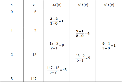
Substituting the values of in (1), we get

Differentiating w.r.to x,

When x = 4,

Exercises 6.1

1. Find the value of and hence from the following table:

   x	0	1	2	3	4	5
   y	0	0.25	0	2.25	16	56.25

2. The following table gives the velocity of a body at t. Find its derivative at t = 1.1

   t	1.0	1.1	1.2		1.4
   v	43.1	47.7	52.1	56.4	60.8

3. Find (0) and (0) from the following table:

   x	0		2	3	4	5
   y	4	8	15	7		2

4. Find the first and second derivatives at x = 1.5 if

   x	1.5	2	2.5	3	3.5	4
   f(x)	3.375	7.000	13.625	24.000	38.875	59.000

5. Find of the function, given by the following table at the point x = 1.1

   x	1	1.2	1.4	1.6	1.8	2
   f(x)	0	1.28	0.544	1.296	2.432	4

6. Given the following table of values of x and y.

   x	1		1.10	1.15	1.20	1.25	1.30
   y	1	1.0247	1.0488		1.0954	1.1180	1.1401

   Find and at (a) x = 1, and (b) x = 1.25

7. Find the derivative of f (x) at x = 0.4 from the following table:

   x	0.1	0.2	0.3	0.4
   f(x)	1.10517	1.22140	1.34986	1.49182

8. Given the following table:

   x	1.96	1.98	2	2.02	2.04
   y	0.7825	0.7739	0.7651	0.7563	0.7473

   Find at x = 2.03.

9. Find the values of (3) and (3) from the following data, using the method Newton’s divided difference formula for interpolation.

   x	1	3	5	7	9
   f(x)	85.3	74.3	67.0	60.5

10. Find the values of (4) and (4) from the following data using Newton’s divided difference formula:

    x	1	2	4	8	10
    f(x)	0	1	5	21	27

11. Find the values of at x = 2, x = 5 from the following data:

    x	0	1	3	6
    f(x)	18	10	−18	40

12. Find the values of and at (i) x = 51 and (ii) x = 55 from the following data:

    x	50	51	52	53		55	56
    y	3.6840	3.7084	3.7325	3.7563	3.7798	3.8030

13. Find the values of (23) and (23) from the following data:

    x	15	17	19	21	23	25
    f(x)	3.873	4.123	4.359	4.583	4.796	5

14. Find the first and second derivatives of at (i) x = 15 and (ii) x = 25 from the following data:

    x	15	17	19	21	23	25
    	3.873	4.123	4.359	4.583	4.796	5.000

15. Find and at x = 51 from the following data:

    x	50	60	70	80	90
    y	19.96	36.65	58.81	77.21	94.61

Answers 6.1

(1) (2) 45.16

(3) −27.9, 117.67 (4)

(5) (6) (a) 0.5005, −0.2732;

(6) (b) 0.4473, −0.1583

(7) 1.4913 (8)

(9) (10) 0.58, 1.029

(11) −15.444, 28.889 (12) (i) 0.02425, −0.0003

(12) (ii) 0.02305, −0.0003

(13) (i) 0.1040 (ii) −0.0023 (14) (i) 0.1292, −0.0046,

(15) (ii) 0.1004, −0.0029

(16)

6.2 Maxima and minima of tabulated function

In calculus, for a differentiable function f, local maximum and minimum are obtained by solving and testing the sign of for the solutions of .

If for a solution then has a maximum at

if for a solution then has a minimum at

In the case of tabulated data, we represent it by a suitable interpolation formula and proceed as above.

Suppose the data give rise to a constant column in the difference table, we represent by Newton’s forward formula.

Otherwise, we have to choose a suitable value as the origin and represent by an appropriate interpolation formula.

Suppose the given values increase up to x₁ and then decrease, then in the neighbourhood of x₁ maximum occurs.

Choose x₁ as the origin and . Since u is small higher powers of u may be neglected and so we may take the formula in u upto third or fourth degree and proceed as above to get the maximum or minimum value of the function.

WORKED EXAMPLES

Example 1

Find the maximum and minimum values of y tabulated below:

x	–2	–1	0	1	2	3	4
y	2	–0.25	0	–0.25	2	15.75	56

Solution

The given values of x and y are

x₀ = −2, x₁ = −1, x₂ = 0, x₃ = 1, x₄ = 2, x₅ = 3, x₆ = 4

y₀ = 2, y₁ = −0.25, y₂ = 0, y₃ = −0.25, y₄ = 2, y₅ = 15.75, y₆ = 4

Let us form the difference table

x	y
−2	2
−2.25
−1	−0.25	2.50
0.25	−3
0	0	−0.50	6
	3
1	−0.25		6
2.25
2	2	11.50
13.75	15
3	15.75	26.50
40.25
4	56

Since the fourth differences are constant, the given function is a polynomial of degree 4 in x

We shall represent the function by Newton’s forward formula

where

Choose the origin as x₀ = 0, h = 1 ∴ u = x

<img arr.eps>

(1)

For maximum or minimum

When x = 0,

∴ y is maximum when x = 0 and the maximum value = 0

When x = −1,

∴ y is minimum when x = −1 and the minimum value = - 0.25

When x = 1,

∴ when x = 1, y is minimum and the minimum value = - 0.25

Example 2

For what values of x is the following tabulated function a minimum?

x	3	4	5	6	7	8
f(x)	-205	-240	-259	-262	-250	-224

Solution

we observe from the given table that the functional values keep on decreasing upto −262 (ie upto x = 6) and then increases

So, the minimum occurs in the neighbourhood of x = 6

∴ choose the origin as Here h = 1

Since the origin 6 is near the middle of the table, a central difference formula is used

∴ we use Stirling’s formula for the given data.

Now we form the difference table

Stirling’s formula in u is

Differentiating w.r. to u, we get

For minimum of

= 30.30795 or − 0.30795

When u = 30.30795, x − 6 = 30, 30795

⇒ x = 36.30795

which is outside the table and so we reject it.

∴ u = − 0.30795 gives the minimum

∴ x − 6 = − 0.30795

⇒ x = − 0.30795 + 6 = 5.6921

∴ the function is minimum when x = 5.6921

Note: When u = − 0.3075, 15 = 15.3075 > 0

∴ y is minimum when u = − 3075

⇒ x = 5.6921

Example 3

Find the appropriate maximum value of given the following table.

x	1	2	3	4	5	6	7
	4774	4968	5104	5183	5208	5181	5104

Solution

we observe from the given table that the functional values keep on increasing up to 5208 ie up to x = 5 and then decreases.

So, the maximum occurs in the neighbourhood of x = 5

Choose the origen as x₀ = 5. Here h = 1

∴

We can use Stirling’s formula or Bessel’s formula

We use Bessel’s formula.

Now we form the difference table

x	u = x − 5
1	−4	4774
194
2	−3	4968	-58
136
3	−2	5104	−57	2
79	3
4	−1	5183	−54	−1
25	2
5	0	5208	-52	0
	-27	2
6	1	5181	-50
−77
7	2	5104

= 5184.5 − 27 − 25.5(u² − u)

⇒ (1)

∴

For a maximum or minimum of

But u = 52.032 is outside the table and so we reject it

∴ u = −0.0321

⇒ x − 5 = −0.321

⇒ x = 5 −0.0321 = 4.9679

To find the maximum value f (4.9679), put u = − 0.0321 in (1)

∴ maximum value = −26 (−0.0321)²−1.6667(−0.0321) + 5208

= −0.00001103 − 0.02679066 + 0.05350107 + 5208

= 5208.0267

Example 4

Find the maximum and minimum values of tabulate below.

x	0	0.2	0.4	0.6	0.8	1	1.2	1.4
	1.23	0.32	-0.35	-0.05	0.08	1.25	1.01	0

Solution

Since maximum and minimum values are required, we shall first form the difference table to see any difference column has constant values.

Now we form the difference table

Since the values are not equal in the last column, we find the maximum and the minimum separately using stirling’s formula.

We observe that the functional values decreases upto −0.35 ie. upto x = 0.4 and then increases.

So, the minimum occurs in the neighbourhood of x = 0.4

So, we use the origin as x₀ = 0.4. Here h = 0.2

<img ellipse.eps>

 

By Stirling’s formula,

(1)

Differentiating (1) w.r. to u, we get

For maximum or minimum

we shall find the value of u by successive approximation method

⇒ <img ellipse.eps>

First approximation is

u₁ =

Second approximation is

Third approximation is

Fourth approximation is

⇒

Since u₃ u₄ for four places of decimals,

we take

when x = 0.4273, y is minimum

substituting u = 0.1363 in (1), we get

the minimum value

∴ maximum value -0.3602

Now we shall find the maximum value.

We observe that values increase upto 1.25 ie upto x = 1, and then decrease

So, the maximum occurs in the neighbourhood of x = 1

Choose the origin as x₀ = 1. Here h = 0.2

Now we form the difference table

We use Stirling’s formula to find u.

Stirling’s formula is

(2)

For maximum

We find u by successive approximation method.

First approximation is

Second approximation is

Third approximation is

Fourth approximation is

Fifth approximation is

Since u₄ = u₅ for four place of decimals, we take

u = 0.3490

Substituting u = 0.349 in (2), we get the maximum value.

The maximum value = 0.1288 (0.349)⁴ − 0.15(0.349)³ - 0.8338 (0.349)²

+ 0.615(0.349) + 1.25

= 0.001911 − 0.006376 − 0.10156 + 0.21464 + 1.25

= 1.3586

Exercises 6.2

1. Find the minimum value of from the following table.

   x	0	1	2	3	4	5
   	58	43	40	45	52	60

2. For what value of x, the following tabulated function of x is minimum?

   x	0.2	0.3	0.4	0.5	0.6	0.7
   y	0.918	0.898	0.887	886	0.894	0.909

3. For what value of x is the following tabulated function maximum?

   x	0.2	0.3	0.4	0.5	0.6	0.7
   y	8.3		8.7	6.4	2.4	4.6

4. From the table below determine the value of x for which the function is a maximum.

   x	3	4	5	6		8
   y	208	240	259	262	250	224

5. Find the maximum and minimum values of the function from the following table.

   x		1.1	1.2	1.3	1.4	1.5	1.6	1.7
   	−11	−12.106	−13.008	−13.62	−14.104	−14.250	−14.096	3.018

   [Hint: Third difference will be constant, use Newton’s forward difference formula]

6. Find the maximum and minimum values of y tabulated below.

   x	0		3	4	5
   y	0	0.25	0.10	−0.20	3

Answers 6.2

1. Minimum at x = 1.7889

   Minimum value = 39.8027

2. Minimum at x = 0.496

   Minimum value = 0.8852

3. Maximum at x = 0.308
4. Maximum at x = 5.695
5. Maximum at x = 1

   Maximum value = 17

   Minimum at = 1.5

   Minimum value = −14.25

6. Maximum at x = 1.0728

   Maximum value = 0.2561

   Minimum at x = 3.4363

   Minimum value = −0.4.894

Short Answer Questions

1. Find at x = 1 from the following table.

   x	1	2	3	4
   y	1	8	27	64

2. State Newton’s formula to find using the forward differences.
3. If , is given for x = 0, 0.5, 1, ... , then show by numerical differentiation that .
4. Write down the formula for using Newton’s backward difference formula.
5. For a function given by the table find at x = 3.

   x	3	4	5
   y	36	73	134

6. The following data gives the velocity of a particle for 15 seconds at an interval of 5 seconds. Find the initial acceleration using the entire data.

   Time t (secs)	0	5	10	15
   Velocity v (m/sec) v	0	3	14	69

7. The following data gives the corresponding values of pressure and specific volume of a super heated steam.

   V	2	4	6	8
   P	105	43.7	25.3	16.7

   Find the rate of change of pressure w.r.to volume when V = 2.

8. For the data

   x	0	3	4
   y	12	6	8

   Find at x = 1.

9. If u₆ = 1.556, u₇ = 1.690, u₉ = 1.908 find when x = 8.
10. Assuming Bessel’s interpolation formula, prove that

    

11. Assuming Bessel’s formula prove that