7.0 INTRODUCTION

We know that can be evaluated if there exists a differentiable function F such that in However, in applications we come across integrals of the form which cannot be evaluated in closed form or analytical form. Sometimes is given by a set of recorded values

In such cases we use the method of numerical integration.

Numerical Integration is the process of evaluating a definite integral from a set of tabulated values of the integrand , which is not known or complicated. This process is known as mechanical quadrature.

Geometrically, represents the area bounded by the curve and the x-axis between and

The process of Numerical integration is carried out by first approximating the integrand by an interpolating polynomial and then integrating between the given limits. Thus is approximately equal to

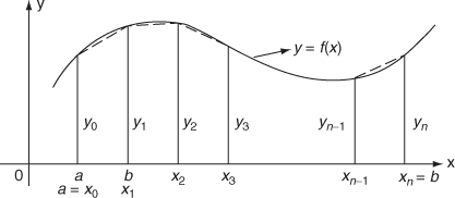
We shall now derive a general quadrature formula for equidistant ordinates based on Newton’s forward difference formula.

7.1 A GENERAL QUADRATURE FORMULA OR NEWTON-COTES QUADRATURE FORMULA

Let be the integral to be evaluated.

Divide into n subintervals each of equal length

Let be the points of division of so that

Let be the values of the function at the points respectively.

Newton’s forward difference formula for this data is

where

When

∴

(1)

From this general formula we deduce some important quadrature formulae by putting

7.2 TRAPEZOIDAL RULE

The trapezoidal rule is

Newton-Cotes formula is

(1)

Put n = 1 in (1), then we get

Because in this case, we have only two points and of x and the values y₀ and y₁ of y, the second and higher differences are zero

This is known as trapezoidal rule. This is also known as general form of Trapezoidal rule or composite trapezoidal rule.

7.2.1 Geometrical meaning

The integral represents the area bounded by the curve the x-axis and the ordinates and

In trapezoidal rule the curve is replaced by n straight line segments joining the points and and and

The sum of the areas of these trapeziums is taken as the area under the curve.

Hence the name Trapezoidal rule.

WORKED EXAMPLES

Example 1

Dividing the range into 10 equal parts, find the approximate value of by Trapezoidal rule.

Solution

Given .

Here The interval is

The interval is divided into 10 equal parts.

∴

The values of x are .

We shall find the values of at these points

By Trapezoidal rule,

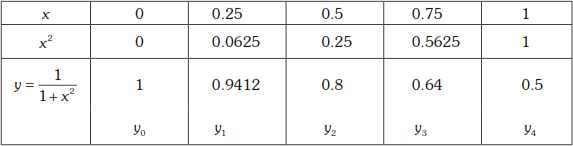
Example 2

Evaluate using trapezoidal rule taking h = 0.25.

Solution

Given

Here

∴ the ponits are x₀ = 0, x₁ = 0.25, x₂ = 0.5, x₃ = 0.75,

x₄ = 1, x₅ = 1.25, x₆ = 1.5, x₇ = 1.75, x₈ = 2,

We shall find the values of y and they are given by the table below.

By Trapezoidal rule,

Example 3

A rocket is launched from the ground. Its acceleration is registered during the first 80 seconds and it is in the table below. Using trapezoidal rule find the velocity of the rocket at t = 80 secs.

t secs	0	10	20	30	40	50	60	70	80
f : cm/sec2	30	31.63	33.34	35.47	37.75	40.33	43.25	46.69	40.67

Solution

Let v and a be the velocity and acceleration at time t

Given a = f(t) cm/sec²

∴

We use trapezoidal rule to find the velocity v, when t = 80 secs

∴

They given table is

Here n = 8, and h = 10

By Trapezoidal rule,

∴ when t = 80 secs, the velocity is v = 3037.95 cm/sec

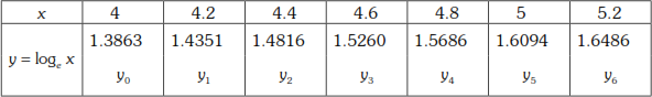
Example 4

Evaluate using the following table by trapezoidal rule.

x	4	4.2	4.4	4.6	4.8	5	5.2
	1.3863	1.4351	1.4816	1.5261	1.5686	1.6094	1.6487

Solution

The given table is

Here

By Trapezoidal rule,

Example 5

Evaluate dividing the range into 4 equal parts by Trapezoidal rule.

Solution

Given

Here . Interval is

The interval is divided into 4 equal parts.

∴

∴ the points are

We find the values of at these points and they are given by the table below.

By Trapezoidal rule,

7.3 SIMPSON’S RULE OR SIMPSON’S RULE

Simpson’s rule is

Proof: In the general quadrature formula put .

Then the interval is to . So, the points are , , and the values of y are respectively.

Since three values are given, third and higher differences are zero

⇒

Similarly,

Adding, we get

where n is a multiple of 2.

That is the number of sub-intervals should be 2, 4, 6, 8, . . .

This formula is called Simpson’s rule or Simpson’s rule.

It is also known as composite Simpson’s rule.

7.3.1 Geometrical meaning

In Simpson’s method in each interval where n is even, the curve is replaced by a second degree polynomial or parabola.

That is the curve is replaced by arcs of parabola. So, the area under the curve is taken as sum of the areas under the parabolic arcs.

The dotted line is the graph of and the thick lines are various parabolae.

WORKED EXAMPLES

Example 1

Evaluate by dividing the interval into eight equal parts and hence find the approximate value of

Solution

Given

Here

The interval is [2, 10].

We divide the interval into eight equal parts ∴

So, we use Simpson’s rule to find

The points are

The values of y at these pernts are given by the table below.

By Simpson’s formula,

By direct integration,

∴

Note: But the value of correct upto 5 places.

So, we find Simpson’s formula gives the value correctly to 3 decimal places.

Example 2

A rocket is launched from the ground. Its acceleration is registered during the first 80 seconds and it is in the table below. Using Simpson’s rule, find the velocity of the rocket at t = 80 secs.

t secs	0	10	20	30	40	50	60	70	80
f : cm/sec2	30	31.63	33.34	35.47	37.75	40.33	43.25	46.69	40.67

Solution

Let v be the velocity of the rocket at t secs,

∴

When

Given table is

Here n = 8, h = 10

By Simpson’s rule,

∴ when t = 80 secs, the velocity is v = 3052.77 cm/sec

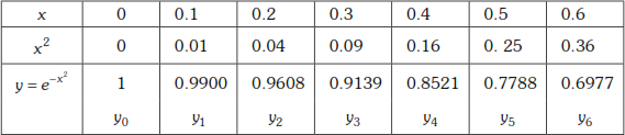
Example 3

Use Simpson’s rule to find by taking seven ordinates.

Solution

Given

Here

The interval is [0, 0.6] and divide the interval into six equal parts and so there will be seven ordinates.

The points are

Now we shall find the values of at these points are given by the table below.

By Simpson’s rule,

Example 4

The following table gives the velocity u of a particle at time t:

t (secs)	0	2	4	6	8	10	12
v (m/sec)	4	6	16	34	60	94	136

Find the distance moved by the particle in 12 secs and also the acceleration at t = 2 secs.

Solution

Let s be the distance moved at time t

Let v and a be the velocity and acceleration at time t.

We know that velocity and acceleration

∴

When t = 12 secs, the distance travelled , where y = v

The values of y are given by the table.

By Simpson’s rule,

∴ when t = 12, distance moved is s = 552 meters

We want acceleration when t = 2 sec.

⇒

ie. we want to find the derivative of v.

So, we form the difference table.

Newton’s forward formula is

where

When

∴ when t = 3 secs, the acceleration is a = 3 m/sec²

Example 5

Evaluate using Simpson’s rule, given that

x	0	1	2	3	4	5	6
	1	0	1	4	9	16	25

Solution

Let

Here

The number of intervals is 6 and h = 1 ∴ n = 6, a multiple of y₂.

So, we can use Simpson’s rule

The points are

The values of y are given by the table below.

By Simpson’s rule,

Example 6

A solid of revolution is formed by rotating about the x-axis, the area between the x-axis and the lines x = 0, x = 1 and a curve through the points with the following coordinates.

x	0.0	0.25	0.50	0.75	1
y	1	0.9896	0.9589	0.9089	0.8415

Estimate the volume of the solid formed using Simpson’s rule.

Solution

The volume v of solid of revolution about the x-axis, the area between the curve the x-axis and the lines x = 0 and x = 1 is

The interval [0, 1] is divided into four equal parts with h = 0.25

∴ n = 4, a multiple of 2.

So, we can use Simpson’s rule to find the required volume

The points are

The values of are given by the table below.

By Simpson’s rule,

∴ volume v = 2.8193 cubic units

7.4 Simpson’s rule

Simpson’s rule is

Proof: We derive the formula using the general quadrative formula.

In the general quadrature formula, put n = 3

Then the interval is and the four values of y are

So, the fourth and higher differences are zero

Now

∴

Similarly,

Adding we get

where n is a multiple of 3.

This formula is called Simpson’s rule.

This formula is also known as Composite Simpson’s rule.

Note: For applying Simpson’s rule, the number of sub-intervals of should be a multiple of 3. Usually we divide into 6 or 9 sub-intervals.

7.4.1 Geometrical Meaning

In Simpson’s rule, in each interval,

Where n is a multiple of 3, the curve is replaced by are of a cubic polynomials.

So, the area under the curve is taken as the sum of the areas under the arcs of the cubic polynomial.

The dotted line is the curve and the thick lines are various arcs of the cubic polynomials.

WORKED EXAMPLES

Example 1

Evaluate taking 7 ordinates by applying Simpson’s rule. Deduce the value of log_e2.

Solution

Let

Here

Since the number of ordinates is 7, the number of subintervals is 6.

∴ the points are

The values of y are y_0, y_1, y_2, y_3, y_4, y_5, y₆ and they are given by the table below.

By Simpson’s rule,

But

Example 2

A curve is drawn to pass through the points given by the following table.

x	1	1.5	2	2.5	3	3.5	4
y	2	2.4	2.7	2.8	3	2.6	2.1

Using Simpson’s rule, estimate the area bounded the curve, the x-axis and the lines x = 1, x = 4.

Solution

Required area is A =

The given table is

Number of intervals is 6 and h = 0.5

∴ n = 6, a multiple of 3.

So, we can use Simpson’s rule to find the required area bounded by the x-axis and the lines x = 1, x = 4,

By Simpson’s rule,

A =

∴ area is

Example 3

A river is 60 ft wide. The depth y feet at a distance x ft from one bank is given by the following table.

x	0	10	20	30	40	50	60
y	0	4	7	9	12	15	14

Find approximately the area of cross-section.

Solution

The area of the cross-section is

The given table is

Number of intervals is 6 and h = 10

∴ n = 6, a multiple of 3.

So, we use Simpson’s rule to find the area of the cross-section.

By Simpson’s rule,

∴ area of the cross-section is A = 547.5 sq.ft

Example 4

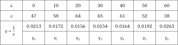
The velocity v of a particle at a distance s from a point on its path is given by the table

s.ft	0	10	20	30	40	50	60
v ft/sec	47	58	64	65	61	52	38

Estimate the time taken to travel 60 ft by using Simpson’s rule. Compare the result with Simpson’s rule.

Solution

Let s be the distance travelled and v be the velocity at time t secs.

∴ We know that velocity

∴

∴ the time taken to travel s = 60 ft is . Let

We shall form the table of values of y.

Here h = 10 and n = 6, even

By Simpson’s rule,

Here h = 10,

∴

By Simpson’s rule,

∴ the time taken by the particle to travel 60 ft by the two methods are equal, correct to 2 places of decimals.

Example 5

Evaluate by using (i) direct integration (ii) Trapezoidal rule (iii) Simpson’s rule (iv) Simpson’s rule.

Solution

Let

Here

Let

The parts are

(ii) Trapezoidal rule

By Trapezoidal rule,

(iii) Simpson’s rule

By Simpson’s rule,

(iv) Simpson’s rule

By Simpson’s rule,

(i) By direct integration

7.5 BOOLE’S RULE

Boole’s rule is

Proof: We derive the formula using the general quadrature formula

In the general quadrature formula, put then the interval is and the five values of y are

So, the fifth and higher differences are zero.

Now

Similarly,

Adding all these integrals, we get

where n is a multiple of 4

ie the number of sub-intervals should be 4, 8, 12, ...

This formula is called Boole’s formula.

This formula is also known as composite Boole’s formula.

WORKED EXAMPLES

Example 1

Evaluate using Boole’s rule with

Solution

Let

Here

∴ number of sub-intervals is 4,

So, we can use Boole’s rule.

The points are

The values of y are y₀, y₁, y₂, y₃, y₄ and they are given by the table below

By Boole’s rule,

Example 2

Use Boole’s rule to estimate approximately the area of the cross-section if the river is 80 ft wide, the depth d ft at a distance x from one bank being given by the following table.

x	0	10	20	30	40	50	60	70	80
d	0	4	7	9	12	15	14	8	3

Solution

Required area is where

Given table is

Number of interval is 8

∴ n = 8, a multiple of 4 and h = 10

So, we can use Boole’s rule to find the required area.

By Boole’s rule,

∴ the area of the cross–section is 708 sq.ft

Example 3

The velocity v of a particle at distance x from a point on its path is given below

	0	10	20	30	40
	45	60	65	64	42

Find the time taken to cover the distance of 40 meters.

Solution

Let v be the velocity at time t.

Since x is given as the distance covered by a particle at time t, we know the velocity is

∴ the time taken to travel x = 40 is

The values of y are given by the table below

The number of value is 4 and h = 10 ∴

So, we can use Boole’s rule to find

By Boole’s rule,

∴ the time taken to travel the distance 40 metres 0.6846 minutes

= 0.6648 × 60 secs = 41.076 secs

7.6 WEDDLE’S RULE

Weddle’s rule is

Proof: = 6, then the interval is is and the seven values of y are involved.

So, the seventh difference and higher difference are zero.

To rewrite the formula conveniently, replace by , as the error involved is negligible for small values of h.

⇒

Similarly,

Adding all these integrals, we get

where n is the number of intervals and it is a multiple of 6.

That is the number of sub-intervals should be 6, 12, 18, …

This is known as Weddle’s rule.

WORKED EXAMPLES

Example 1

Evaluate by using Weddle’s rule.

Solution

Let (1)

Here

Divide the interval [0, 6] into 6 equal intervals.

∴ the number of sub-intervals is 6, a multiple of 6.

∴ and

So, we can use Weddle’s rule to find (1)

The points are

The values of y are y₀, y₁, y₂, y₃, y₄, y_5, y₆ and they are given by the table below

By Weddle’s rule,

Example 2

A curve is drawn to pass through the points given by the following table.

x	1	1.5	2	2.5	3	3.5	4
y	2	2.4	2.7	2.8	3	2.6	2.1

Using Weddle’s rule, estimate the area bounded by the curve, the x-axis and the lines x = 1, x = 4.

Solution

The area bounded by the curve the x-axis and the lines is

The interval [1, 4] is divided into 6 equal parts with

∴ n = 6, a multiple of 6

So, we can use Weddle’s rule to find

The points are

The values of y are y₀, y₁, y₂, y₃, y₄, y₅, y₆ and they are given by the table below.

By Weddle’s rule,

∴ the area is 7.74 sq. units

Example 3

Use Weddle’s rule to evaluate the approximate value of given that

x	4.0	4.2	4.4	4.6	4.8	5	5.2
	1.3863	1.4351	1.4816	1.5260	1.5686	1.6094	1.6486

Compare it with exact value.

Solution

Let (1)

Here

The interval is (4, 5.2) and it is divided into 6 equal parts with h = 0.2

∴

So, we can use Weddle’s rule to find (1).

The points are

The values of y are y₀, y₁, y₂, y₃, y₄, y₅, y₆ and they are given by the table below.

By Weddle’s rule,

By direct integration,

∴ the actual value is 1.8278

By Weddle’s rule, the value is 1.8278

∴ error is zero.

Example 4

The velocity of the particle at a distance s from a point on its path is given by the table below.

s (metres)	0	10	20	30	40	50	60
v (m/sec)	47	58	64	65	61	52	38

Estimate the time taken to travel 60 meters by (i) Simpson’s rule

(ii) Simpson’s rule

(iii) Weddle rule.

Solution

Let s be the distance travelled and v be the velocity at time t.

We know the velocity

∴ the time taken to travel 60 ft is

The values of y are y₀, y₁, y₂, y₃, y₄, y₅, y₆ and they are given by the table below

Number of intervals is 6 with h = 10

1. Simpson’s rule,

   

   

2. By Simpson’s rule,

   

3. By Weddle’s rule,

   Since n = 6, we can use weddle’s formula.

   

   ∴ by the three methods, the time taken to travel the distance is equal, correct to two places of decimal.

7.7 ERROR IN NUMERICAL INTEGRATION FORMULAE

7.7.1 Error in Trapezoidal Rule

Trapezoidal rule is

where are the values of at

where and

Taylor’s series expansion for f (x) about x₀ is

(1)

(2)

where

Area of the trapezium in is

⇒ (3)

(4)

∴ The principal part of error in (x₀, x₁) is

Similarly principal part of error in (x₁, x₂) is etc.

error in is

∴ total error E is given by

If , then

Hence the total error in Trapezoidal rule is of order h²

7.7.2 Error in Simpson’s Rule

Simpson’s rule is

where is even, are the values of y = f(x) at

Taylor’s series expansion of f(x) about x₀ is

(1)

(2)

But by Simpson’s rule, area in [x₀, x₂] is (3)

Putting x = x₁ in (1), we have

∴

Putting in (1), we have

∴

Substituting for y₁ and y₂ in (3) we get

(4)

∴

Omitting h⁶ and higher powers, the principal part of error in is and so on.

the total error

, where

∴

In the same way, we can find the error in the quadrature formulae. We shall indicate the principal error in each formula

Error in Simpson’s rule

The principal error in the interval is

Error in Boole’s rule

The principal error in the interval is

Error in Weddle’s rule

The principal error in the interval is

Exercises 7.1

1. (1) Evaluate using
   1. (i) Trapezoidal rule (ii) Simpson’s rule with
   2. (iii) Simpson’s rule with
2. (2) Evaluate using the following data.

   x	4	4.2	4.4	4.6	4.8	5	5.2
   	1.3863	1.4351	1.4816	1.5261	1.5686	1.6094	1.6487

   1. (i) by Trapezoidal rule (ii) by Simpson’s rule
   2. (iii) by Simpson’s rule
3. (3) Using the following table evaluate by (a) Trapezoidal rule (b) Simpson’s rule.

   x	0	0.5	1.0	1.5	2.0
   y	0.399	0.352	0.242	0.129	0.054

4. (4) Evaluate taking i = 0.1 by 9
   1. (a) Trapezoidal rule
   2. Simpson’s rule
5. (5) Evaluate using
   1. (i) Trapezoidal rule
   2. Simpson’s rule
6. (6) Evaluate by
   1. (i) Trapezoidal rule
   2. Simpson’s rule
7. (7) Evaluate by Simpson’s rule with h = 0.1.
8. (8) Evaluate using Simpson’s rule with h = 0.25 and hence reduce the value of
9. (9) Evaluate
10. Using Simpson’s rule with h = 0.2. Compare the results by integration.
11. Evaluate by Simpson’s rule.
12. Evaluate by Simpson’s rule.
13. Evaluate by Boole’s rule.
14. Evaluate by Boole’s rule.
15. Evaluate by Boole’s rule with 13 ordinates.
16. The following gives the velocity v of a particle at time t..

    t in hrs	0	0.25	0.5	0.75	1	1.25	1.5	1.75	2
    velocity v km/hr	6	7.5	8	9	8.5	10.5	9.5	7	6

    Find the distance travelled in 2 hours.

17. Evaluate using Weddle’s rule
    1. (i)
    2. (ii)
18. Evaluate by Weddle’s rule with 7 ordinates and reduce the value of log_e2.
19. A curve is drawn to pass through the points given by the following table

    x	1	1.5	2	2.5	3	3.5	4
    y	2	2.4	2.7	2.8	3	2.6	2.1

    using Weddle’s rule, estimate the area bounded by the curve, the x-axis and the lines x = 1, x = 4.

Answers 7.1

1. 0.7854, 0.7854, 0.7854 (2) 1.82765, 1.82784, 1.82785
2. 0.475, 0.477 (4) 0.6686; 0.6321
3. 115, 98 (6) 1.4108; 1.3662
4. 0.5351 (8) 0.3108
5. 4.05214 (10) 1.3571
6. 1.3571 (12) 1.8278
7. 3.1067 (14) 0.0549
8. 0.8236 (16) 16.68 km
9. (i) 4.05145 (ii) 0.5051 (18) 0.6932
10. 3.032

7.8 ROMBERG’S METHOD FOR INTEGRATION

We have seen different formulae for numerical integration obtained by the finite difference methods. Of the three formulae trapezoidal rule, Simpson’s rule and Simpson’s rule, Simpson’s rule gives the best result.

A method due to L.F Richarson known as Richardson’s deferred approach to the limit provides a method to improve the accuracy of the approximate values of definite integrals obtained by finite difference methods. This technique is known as Romberg’s integration.

7.8.1 Romberg’s Integration Formula Based on Trapezoidal Rule

Let

Let I₁, I₂ be two values of I by trapezoidal rule with subintervals of width h₁, h₂ and let E₁, E₂ be their corresponding errors. Let

Then

and

Since are both largest values of we can assume and are nearly equal.

But I = I₁ + E₁ and also I = I₂ + E₂

which is a better approximation of I than I₁ and I₂.

This method is called Richardson’s deferred approach to the limit.

To evaluate I systematically, we take

(1)

This is known as Romberg’s formula.

The formula (1) is obtained by trapezoidal rule twice with width of intervals h and

We again apply trapezoidal rule with width and apply several times halving the intervals. Each time the error is reduced by a factor

Thus we have a sequence of values of I.

I₁, I₂, I₃, I₄, ... are the values with width

Applying (1) for the pairs I₁, I₂; I₂, I₃; I₃, I₄; ... , we get A₁, A₂, A₃, … . which are improved values.

Again applying (1) to the pairs

We get

This systematic refinement of Richardson’s method is called Romberg method or Romberg integration.

WORKED EXAMPLES

Example 1

Evaluate correct to 3 places using Romberg’s method and hence find the value of log_e 2.

Solution

Let

Here

Trapezoidal rule is

We shall find the value of the integral when h = 0.5, 0.25, 0.125

When h = 0.5, the values of y are given by the table below

When the values of y are given by the table below

When the values of y are given by the table below

We shall now use Romberg’s formula for I₁, I₂

Again for I₂ and I₃, we have

Now again applying Romberg’s method with

By direct integration,

∴

Note: We find using calculator log_e 2 = 0.69314718.

So, the answer by Romberg’s method is correct to 4 decimal places.

Example 2

Evaluate by using Romberg’s method correct to 4 decimal places. Hence deduce an approximate value of p.

Solution

Let

Here

Trapezoidal rule is

We shall find the value of I by trapezoidal rule for h = 0.5, 0.25, and 0.125

When h = 0.5, then the values of y are given by the table below

Then

When the values of y are given by the table below

Then

When the values of y are given by the table below.

Then

We shall now use Romberg’s formula for the pairs I₁, I₂.

∴

and for the pair I₂, I₃

So, for 4 decimals the 2 improvements coincide.

∴ the value of I = 0.7854

∴

By direct integration,

Note: From calculator = 3.141592654.

So, the value is correct to 4 places.

Example 3

Evaluate using Romberg’s formula.

Solution

Let

Let

Trapezoidal rule is

We shall find the values of the integral when

When the values of y are given by the table below

When the values of y are given by the table below.

When the values of y are given by the table below.

Applying Romberg’s formula for the pairs and , We get

Again for the pairs I₂, I₃, we get

Again applying Romberg’s formula for we get

∴

Note: By direct integration

So, we find that the value by Romberg’s method is correct.

Example 4

Evaluate using Romberg’s method.

Solution

Let

Here

Trapezoidal rule is

When , we shall find the values of the integral.

When the values of y are given by the table below.

When the values of y are given by the table below.

When the values of y are given by the table below

We shall now use Romberg’s formula for

Again applying Romberg’s method with we get

Since upto 4 places of decimals.

We shall take I = 0.3927

Note:

By direct integration

So, we find that the value by Romberg’s method is correct.

7.8.2 Romberg Integration Formula Based on Simpson’s Rule

Let .

Let be two values of I by Simpson’s rule with sub-intervals width and let be their corresponding errors.

Then

and

where and are largest values of ,

We assume them to be nearly equal.

Suppose and then

But

(1)

This is Romberg’s formula using Simpson’s rule.

Again applying Simpson’s rule with , we get a sequence of values of I.

Let be the values of the integral with width

Applying the formula (1) for the pairs

we get which are improved values of I.

Again applying (1) to the pairs

we get which are still improved values.

This method is called Romberg’s method.

WORKED EXAMPLES

Example 1

Find the value of correct to 4 decimal places using Simpson’s rule and Romberg’s integration.

Solution

Let

Here

Simpson’s rule is

where n is even

We shall find the values of the integral with

When h = 0.5, number of intervals is 2 ∴ n = 2

Since the values of y are given by the table below.

Simpson’s formula is

∴

When h = 0.25, n = 4, even

The values of y are given by the table below.

When h = 0.125, n = 8, even

The values of y are given by the table below.

We now use Romberg’s formula for the pairs and

Also

Since upto five places of decimals, we take

So, the value I,corrected to 4 places of decimal is 1.9461.

Example 2

A certain curve is given by the following points

x	1	2	3	4	5	6	7	8	9
y	0.2	0.7	1	1.3	1.5	1.7	1.9	2.1	2.3

Using Simpson’s rule and Romberg’s formula, find the volume generated by revolving the area bounded by this curve, the x-axis and the ordinates x = 1 and x = 9 about the x-axis.

Solution

Required volume I

Let us evaluate this integral by Simpson’s rule with h = 4, 2, 1

When h = 4, n = 2, even. The values of are given by the table below.

************************************

By Simpson’s formula,

∴

When even

The values of are given by the table below.

By Simpson’s formula,

∴

When , even

The values of y² are given by the table below.

x	1	2	3	4	5	6	7	8	9
y	0.2	0.7	1	1.3	1.5	1.7	1.9	2.1	2.3
	0.04	0.49	1	1.69	2.25	2.89	3.61	4.41	5.29

By Simpson’s formula,

∴

Applying Romberg’s formula for the pairs and we get

Also

Applying Romberg’s formula for

∴ p × I

Example 3

Evaluate using Simpson’s rule and Romberg’s method.

Solution

Let

Here

Simpson’s rule is

Let us evaluate the integral with

When , even

The values of y are given by

x	0	1	2
	0	1	4
	0.25	0.2	0.125

By Simpson’s rule,

∴

When , even

The values of y are given by the table below.

x	0		1		2
	0	0.25	1	2.25	4
	0.25	0.2353	0.2	0.16	0.125

By Simpson’s rule,

∴

When , even

The values of y are given by the table below.

x	0	0.25	0.5	0.75	1	1.25	1.5	1.75	2
	0.25	0.2462	0.2353	0.2192	0.2	0.1798	0.16	0.1416	0.125

By Simpson’s rule,

∴

Now we use Romberg’s formula for the pairs and .

Also

Now applying Romberg’s formula with and , we get

∴

7.9 TWO AND THREE POINT GAUSSIAN QUADRATURE FORMULAE

7.9.0 Introduction

To evaluate the integral we have developed various approximate formulae, namely trapezoidal rule, Simpson’s rule and Simpson’s rule. In these formulae we used the values of the function at equally spaced values of argument x. Here the values of x are predetermined. Gaussian quadrature formula uses the same number of values of but the values of x are not equally spaced and choosing the points suitably we can find an improved estimate of the integral.

Any finite interval [a, b] can be transformed into [–1, 1] by the transformation

and

So, we consider the integral in the form

The general n-point Gaussian quadrature formula assumes an approximation of the form

, where are the points of division of the interval [–1, 1], which are known as nodes and are known as the weights. Since there are 2n unknowns in the relation (1), 2n relations between the variables are necessary and the formula is exact for polynomials of degree Formulae based on this idea are called Gaussian quadrature formulae.

This method is applicable only when f(x) is known explicitly so that the values of the function can be evaluated at any given value of x.

The quadrature formula is derived assuming are the roots of the equation , where is the Legendre polynomial of degree n given by Rodrigue’s formula

We also assume can be expanded as a power series of degree in so that

We shall derive the quadrature formulae when n = 2 and n = 3 which are called the two point quadrature formula and three point quadrature formula respectively.

7.9.1 Two Point Gaussian Quadrature Formula

When n = 2, the two point quadrature formula is

(1)

Where x₁ and x₂ are the roots of P₂ (x) = 0

Since . So is a polynomial of degree 3.

Let

∴ Equating like coefficients we get

The two point quadrature formula is

Note: It is also known as two point Gauss-Legendre formula. It gives good estimate with two functional values.

7.9.2 Three Point Gaussian Quadrature Formula

The three point formula is

(1)

where x₁, x₂, x₃ are roots of P₃ (x) = 0, where P₃ (x) is the Legendre polynomial of degree 3.

Let

To find , we assume f(x) is a polynomial of degree 5, since

Let

Equating like coefficients, we get

(2)

(3)

Substitute in (2), we get

WORKED EXAMPLES

Example 1

Apply Gauss two-point formula to evaluate .

Solution

Let

We know since is even function of x

∴ . Here

Gauss two-point formula is

Example 2

Evaluate by 2-point Gaussian formula.

Solution

Let

First transform the interval into the interval [–1, 1]

For. this, put Here

∴ ∴ <Eqn Eqn1263"/> ∴

When and when

By 2-point Gaussian formula,

But

∴

Example 3

Using three point Gaussian formula, evaluate .

Solution

Let

We have to transform the interval [0.2, 1.5] into the interval [–1, 1]

For this, Put . Here

When and when

Here

Three point quadrature formula is

But

∴

∴

Example 4

Evaluate using 3-point Gauss quadrature formula and compare with the actual value.

Solution

Given

We have to transform the interval [1, 2] into [–1, 1]

For this, Put . Here a = 1, b = 2

∴

When

We know 3-point Gaussian formula is

But

We shall now find the exact value by integration.

Put

When and when

The error is 0.5408 − 0.5404 = 0.0004

Example 5

Evaluate dx by three point Gaussian formula.

Solution

Let dx

First transform the interval [0, 2] into the interval [–1, 1]

But

Example 6

Evaluate using Gaussian (i) two points formula (ii) three point formula.

Solution

Given .

Here

1. (i) Gaussian two point formula is

   

2. (ii) Gaussian three point formula is

   

   

Note: We shall now find the actual value by integration.

∴ Error in 2 point formula = |1.5708 – 1.5| = 0.0708

Error in 3 point formula = |1.5708 – 1.5833| = 0.0125

So the error in 3-point formula is less than the error in 2-point formula.

Example 7

Obtain by using Gauss two point and three point rules.

Solution

Let

Transform the interval [2, 3] into [–1, 1] by the transformation

When and when

∴

∴

1. Two point Gaussian formula is

   

   Now

   

   ∴

2. The three point Gaussian formula is

   ∴

Example 8

Using Gaussian two and three point formulae evaluate .

Solution

Given

First we transform the interval [2, 3] into the interval [–1, 1]

For this, put

When and when

1. (i) Two point Gaussian formula is

   

   

2. (ii) Three point Gaussian formula is

   

Now

∴

Exercises 7.2

1. Evaluate by Romberg’s method with h = 0.1 and h = 0.2 and using Trapezoidalrule.
2. Evaluate by using Romberg’s method taking
3. Calculate using trapezoidal rule with and then Romberg’s formula.
4. From the following data evaluate using Romberg’s method with h=0.8, 0.4

   x	1.8	2	2.2	2.4	2.6	2.8	3	3.2	3.4
   f(x)	6.050	7.389	9.025	11.023	13.464	16.445	20.086	24.533	29.964

5. Evaluate with h = 0.65, 0.325 by Romberg’s method.
6. Evaluate by two point Gaussian formula.
7. Evaluate using two point Gaussian formula.
8. Evaluate by using three point Gaussian formula. Compare with actual value.
9. Evaluate using 3-point Gaussian formula.
10. Evaluate using three point Gaussian formula.
11. Evaluate using two point and three point Gaussian formula.

Answers 7.2

(1) 1.8521 (2) 0.3927 (3) 0.507070

(4) 23.9181 (5) 0.6586 (6) 4.6854

(7) 1.5432, 1.3911 (8) 4 (9) 1.3247

(12) 1.7128 (11) 0.9985

7.10 EULER-MACLAURIN FORMULA FOR NUMERICAL INTEGRATION

Euler-Maclaurin’s formula for integration is

Where and

Derivation: Let

Divide the interval into n equal intervals of width

Let

∴

Adding all these equations, we get

(1)

Since , we define the inverse operator as

∴ (2)

Putting and in (2), we get

(3)

(4)

Substituting for L.H.S. from (1), we get

This is called Euler-Maclaurin’s formula for integration.

Incase higher derivatives are involved, then the formula is

∴

Note: This formula can be rewritten as

This is called Euler-Maclaurin’s formula for summation.

WORKED EXAMPLES

Example 1

Evaluate by Euler-Maclaurin formula for integration. Hence find the value of p and compare with the correct value upto 5 decimals.

Solution

Let

Here

Euler-Maclaurin formula for integration is

∴ (1)

where n = the number of sub-intervals and

Let

The values of x are ,

The values of are given by the table below.

x
0						1
	1	0.97297	0.9	0.8	0.69231	0.59016	0.5

∴ We have

∴

∴

∴

But

Using Calculator

∴ Euler-Maclaurin method gives correct answer upto 5 places of decimal.

Example 2

Find by Euler’s quadrature formula, the value of the integral .

Solution

Let

Here

Euler-Maclaurin’s formula for integration is

where n = the number of sub-intervals and .

Let

The values of x are

The values of are given by table below

x
0					1
	1	0.99920	0.98723	0.93590	0.8021	0.54030

We have

∴

∴

∴

∴

∴

Example 3

Applying Euler-Maclaurin summation formula, evaluate

Solution

Required the sum of

Here

By Euler – Maclaurin formula for summation

We have

∴

and

∴

Example 4

By Euler’s formula prove that the sum of the cubes of the first n natural numbers is .

Solution

We have to prove

Here

By Euler’s formula for summation

We have

∴

∴

7.10.1 Application of Euler-Maclaurin Formula

Stirling’s approximation for factorial

If n is a positive integer, then we know,

∴ (1)

We shall find the sum by Maclaurin’s formula.

Here

Maclaurin’s formula for summation is

∴

(2)

To find C, we use Weddle’s formula, namely

Taking logarithm, we get

∴

As

∴ approximately (from (1) and (2))

∴

Corollary: When n is large are very small and so can be neglected

WORKED EXAMPLES

Example 1

Calculate correct to six places of decimals and hence find the number of digits in 81!

Solution

Stirling’s formula for n! is

Taking log to the base 10,

Put n = 81, we get

∴

Since the integer part is 120, the number of digits in 81! is 121

Example 2

Using Stirling’s approximation for n!, find the number of digits in the value of 100C50.

Solution

Let

Taking log to the base 10, we get

Stirlings formula for n! is

∴ (1)

Put n = 100 in (1), then

Now put n = 50 in (1), then

∴ x = anti log (29.0039)

Since the integral part is 29, the number of digits in 100C₅₀ is 30

Exercises 7.3

(I) Evaluate the following integrals using Euler-Maclaurin formula.

1. correct to fine decimal places.
2. correct to seven decimal places.
3. correct to five decimal places.
4. and hence find the values of p.

(II) Evaluate the following sums.

1. correct to 6 decimals.
2. 
3. correct to 6 places of decimals.
4. 
5. 
6. 
7. 
8. Find the sum of the fourth powers of first n natural numbers.

(III) Using Stirling approximation for factorials, compute to six places of decimals

1. 
2. 
3. 
4. 

Answers 7.3

(I)

1. 2.40011
2. 0.0487902
3. 0.69315
4. 0.7854, π = 3.1416

(II)

1. 0.6956534
2. 0.0049998
3. 0.133137
4. 0.0049988
5. 0.144539
6. 0.11382
7. (7) 0.0008333

(III)

1. 98.233911
2. 615.5999
3. 28.138179
4. 2567.59914

7.11 DOUBLE INTEGRATION

We shall now consider the numerical evaluation of a definite double integral of a function of two independent variables from a set of numerical values of the integrand. The process of computation of double integral of a function of two independent variables is called mechanical cubature.

We have seen in calculus that a double integral with constant limits can be evaluated by integrating w.r.to x first treating y as constant and then integrating w.r.to y. So we can evaluate a double integral by applying trapezoidal rule or Simpson’s rule repeatedly.

7.11.1 Trapezoidal Rule for Double Integral

Let. The region of integration is the rectangle bounded by

the lines x = a, x = b, y = c, y = d in the xy plane.

Divide the interval [a, b] into n equal subintervals of width h at the points

and the interval [c, d] into m equal subintervals of width k at the points

Let

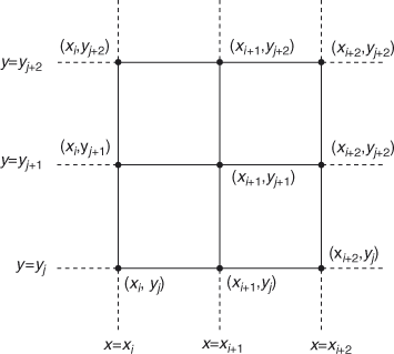
Consider the typical rectangle ABIH over which we shall evaluate the integral

By trapezoidal rule for the inner integral with two values, we get

Again applying trapezoidal rule

(1)

To evaluate , we have to evaluate over the rectangle ACEG, which is the sum of four rectangles.

∴

Using (1) to each of these integrals, we get

More generally, the value of the double integral is

WORKED EXAMPLES

Example 1

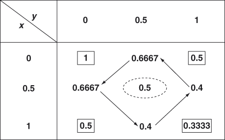
Evaluate by Trapezoidal rule for the following data:

Solution

Let

The given values of x are equally spaced with h = 0.5

The given values of y are equally spaced with k = 1

∴ the Trapezoidal rule for double integral is

The corner values are squared.

Other boundary values are indicated by arrows.

The interior values are inside the dotted curve.

Example 2

Use trapezoidal rule to evaluate taking 4 subintervals.

Solution

Let

Here

Number of subintervals is 4.

∴ the values of x are 1, 1.25, 1.5, 1.75, 2 and the values of y are 1, 1.25, 1.5, 1.75, 2

Similarly

Now we tabulate the values of

∴ the trapezoidal rule for double integral is

The corner values are squared. Boundary values are indicated by arrows. Interior values are inside the dotted curve.

Example 3

Evaluate by Trapezoidal rule.

Solution

Let

Here

We shall take h = 0.5, k = 0.25

∴ the values of x are 0, 0.5, 1 and the values of y are 0, 0.25, 0.5, 0.75, 1.

∴

Similarly

Now we shall tabulate the values of f(x, y)

∴ the Trapezoidal rule for double integral is

[sum of the corner values

+ 2 (sum of other values of on the boundary)

+ 4 (sum of the interior values of]

The corner values are squared.

Other boundary values are indicated by arrows.

The interior values are inside the dotted curve.

Note: The exact value of this double integral is .

So, the error is 0.0087

Example 4

Evaluate by Trapezoidal rule with h = k = 0.25.

Solution

Let

Here

∴ the values of x are 1, 1.25, 1.5, 1.75, 2

and the values of y are 0, 0.25, 0.5, 0.75, 1

Similarly

Now we shall tabulate the value of

∴ the Trapezoidal rule for double integration is

[sum of the corner values

+ 2 (sum of the other values of on the boundary)

+ 4 (sum of the interior values of ]

The corner values are squared.

Other values of f(x, y) on the boundary are indicated by arrows.

The interior values are inside the dotted curve.

∴

Example 5

Evaluate using Trapezoidal rule with h = k = 0.5 and h = k = 0.25. Improve the estimate by Romberg’s formula.

Solution

Let

Here

Case (i) h = k = 0.5

The values of x are 1, 1.5, 2 and the values of y are 1, 1.5, 2

Similarly

We shall tabulate the values of

Trapezoidal rule for double integration is

Case (ii) h = k = 0.25

By worked example 2 page . . . I = 0.3401

Taking the estimates as I₁ = 0.3433 and I₂ = 0.3401

By Romberg’s formula

7.11.2 Simpson’s Rule for Double Integral

Let

We divide [a, b] into an even number of intervals 2n and [c, d] is divided into an even number of intervals 2m.

Applying Simpson’s rule taking 2 intervals in the x-direction and 2 intervals in the y-direction.

Let

The points of division are

∴

The typical sub-rectangles are taken with 2 intervals in x-direction and 2 intervals in y-direction.

Consider

By applying Simpson’s rule in the x-direction, for 2 intervals keeping y-constant to the inner integral we get

Again apply Simpson’s rule to each integral in the y-direction.

This can be extended if the number of intervals is 4 or 6 in each direction applying for every pair of intervals.

WORKED EXAMPLES

Example 6

Evaluate using Trapezoidal rule and Simpson’s rule.

Solution

Let

Here

We shall take h = 0.5, k = 0.5 and thus dividing into 2 intervals each.

∴ the value of x are 0, 0.5, 1 and the values of y are 0, 0.5, 1

∴

We shall tabulate the values

1. (i) Trapezoidal rule for double integral is

   

   

2. (ii) Simpson’s rule for double integral is

   

   

Note: Integrating we get the actual value 2.9525 correct to 4 decimals So we notice that the value of Simpson’s rule is very close to the actual value.

Example 7

Using Simpson’s rule evaluate by taking h = k = 0.5.

Solution

Let

Here

Given

∴ the values of x are 0, 0.5, 1 and the values of y are 0, 0.5, 1.

So the interval is divided into 2 parts.

We shall tabulate the value

Simpson’s rule for double integral is

Note: By integration the actual value is 0.5232 upto 4 places.

Example 8

Evaluate by Simpson’s rule with h = k = 0.25.

Solution

Let

Here and h = k = 0.25

∴ the values of x are 0, 0.25, 0.5 and the values of y are 0, 0.25, 0.5

So the interval is divided into 2 parts.

Similarly,

We shall tabulate the values of f (x, y)

Simpson’s rule of double integral is

Example 9

Evaluate using Simpson rule, given h = k = 0.1.

Solution

Here

Given h = 0.1, k = 0.1

∴ the values of x are 4, 4.1, 4.2, 4.3, 4.4 and the values of y are 2, 2.1, 2.2, 2,3, 2.4

The interval is divided into 4 sub intervals.

Similarly,

f(4.1,2) = 8.2, f(4.1,2.1) = 8.61, f(4.1,2.2) = 9.02,

f(4.1,2.3) = 9.43, f(4.1,2.4) = 9.84,

f(4.2,2) = 8.4, f(4.2,2.1) = 8.82, f(4.2,2.2) = 9.24,

f(4.2,2.3) = 9.66, f(4.2,2.4) = 10.08,

f(4.3,2) = 8.6, f(4.3,2.1) = 9.02, f(4.3,2.2) = 9.46,

f(4.3,2.3) = 9.89, f(4.3,2.4) = 10.12,

f(4.4,2) = 8.8, f(4.4,2.1) = 9.24, f(4.4,2.2) = 9.68,

f(4.4,2.3) = 10.12, f(4.4,2.4) = 10.56

We shall formulate the table value of

We shall rewrite the integral as sum of 4 integrals taking 2 intervals at a time and apply Simpson’s rule

where

∴

Using Simpson’s rule for 2 intervals

∴

∴

Note: Directly integrating we get the exact value as 1.4784. So in this problem Simpson’s formula gives the exact value.

Example 10

Evaluate by Simpson’s rule for double integration.

Solution

Let

Here

Let and

The order of integration is first w.r.to y and then w.r.to x.

The values of x are 4, 4.3, 4.6, 4.9, 5.2 and the value of y are 2, 2.3, 2.6, 2.9, 3.2

The interval is divided into 4 sub-intervals.

We shall tabulate the values of

We shall rewrite the given integral as the sum of four integrals taking two intervals at a time and applying Simpson’s rule

∴

Now

∴

∴

and

∴

∴

Aliter: We shall apply Simpson’s rule to the rows, treating the values 2, 2.3, 2.6, 2.9 and 3.2 as x values and the function values of I row as

Applying for I row, we get the following table:

x	2	2.3	2.6	2.9	3.2
y

∴

Applying for II row, we get the following table.

x	2	2.3	2.6	2.9	3.2
y

Similarly applying Simpson’s rule for III and IV and V rows, we get

Now treating 4, 4.3, 4.6, 4.9, 5.2 as x values and as y values and applying Simpson’s rule we get

Note: By direct integration the actual value of the integral is

Error = 0.123312 – 0.123316 = 0.000004, which is negligible.

Exercises 7.4

• Evaluate using trapezoidal rule taking h = 0.1 and k = 0.8.
• Evaluate using trapezoidal rule with 4 subintervals.
• Evaluate using trapezoidal rule with 4 subintervals.
• Apply Simpson’s rule to evaluate by taking h = 0.2, k = 03.
• Evaluate taking h = k = 0.5 by Simpson’s rule.
• Evaluate using Simpson’s rule by taking . Also find by trapezoidal rule.
• Evaluate using Simpson’s rule with
• Evaluate using
• (i) Trapezoidal rule and (ii) Simpson’s rule with

Answers 7.4

(1) 0.0429 (2) 3.9975 (3) 0.0614

(4) 0.025 (5) 0.0408 (6) 2.0095, 1.7976

(7) 2.1546 (8) (i) –1.7976 (ii) –2.0091

Short Answer Questions

1. Evaluate by Trapezoidal rule, dividing the range into 4 equal parts.
2. When does Simpson’s rule give exact result?
3. Write down trapezoidal rule to evaluate with h = 0.5, function f(x) is unknown.
4. In order to evaluate by trapezoidal rule and by Simpson’s rule, what is the restriction on the number of intervals?
5. What are the errors in trapezoidal and Simpson’s rules of numerical integration?
6. What is the order of error in Simpson’s rule?
7. State the local error term in Simpson’s rule.
8. State Newton’s formula to find using the forward differences.
9. What is the order of the error in trapezoidal rule?
10. Why is trapezoidal rule so called?
11. Write down Simpson’s rule, assuming 3n intervals.
12. What are the truncation errors in Trapezoidal rule and Simspon’s rule?
13. Evaluate using trapezoidal rule by taking
14. Using two point Gaussian quadrature formula, evaluate
15. Evaluate using Gaussian quadrative with 2 points.
16. State Romberg’s integration formula to find the value of using