Search in book...
Toggle Font Controls
Create new playlist

Name your new playlist

Playlist description (optional)
Sign In

Email address

Password

Forgot Password?

or

Continue with Facebook

Continue with Google
Sign Up

Full Name

Email address

Confirm Email Address

Password

or

Continue with Facebook

Continue with Google

Chapter 9

Discrete Element Methods

Abstract

The discrete element method (DEM), also know as the distinct element method, is a numerical method for modeling the micromechanics and dynamics of particle systems (i.e., assemblies of individual particles). It was initially developed for analyzing soil mechanics and geotechnical problems and has been adapted and used extensively to study the mechanics of bulk materials and to model powder handling and processing. In DEM, a bulk material is treated as a system consisting of many individual solid particles that interact with each other according to certain interaction laws, depending on material and interfacial properties. In this chapter, the principle of DEM is introduced, techniques developed for modeling contact detection and interaction are discussed, with a brief description of various contact models used in DEM. In addition, methods for determining the time step used in DEM and some DEM parameters are explained. Furthermore, approaches to analysis of the data generated from DEM modeling are introduced, and some typical applications of DEM are presented.

Keywords

Contact detection; Contact modeling; Coordination number; Discrete element method (DEM); Discrete particle method; Electrostatics; Force transmission; Heap formation; Hopper flow; Mixing; Packing density distribution; Particle packing; Powder compaction; Powder flow; Radial distribution function (RDF); Segregation; Structural anisotropy; Voronoi cell

The discrete element method (DEM), also know as the discrete particle method, is a numerical method for modeling micromechanics and dynamics of particle systems (i.e., assemblies of individual particles). It originated with the seminal paper of Cundall and Strack on “a discrete numerical model for granular assemblies” in 1979. Since then, it has been significantly advanced by many researchers. Although DEM was initially developed for analyzing soil mechanics and geotechnical problems, it has been adapted and used extensively to study the mechanics of bulk materials and to model powder handling and processing.

In DEM, a bulk material is treated as a system consisting of many individual solid particles that interact with each other according to certain interaction laws, depending on their material and interfacial properties. The particles may have complex shapes, and significant advances have been made in modeling irregular-shaped particles using DEM in recent years. More usually, though, particles have been modeled as disks in 2D or spheres in 3D in most DEM codes. The reason that spheres are often used in DEM modeling is clearly because rigorous interaction models based upon contact mechanics are well established for spheres, as discussed in Chapter 8. Moreover, for spherical particles, contact detection and modeling can be easily implemented and efficiently executed so that a large number of particles (say >1,000,000 particles) can be modeled in a reasonable timescale.

9.1. Hard-Sphere and Soft-Sphere DEMs

The core of DEM is to model the interactions between particles, which are generally dynamic processes, and an explicit time-dependent finite difference technique (see Section 9.2.1) is normally used to analyze their progressive motion. According to the choice of particle interaction model used, DEM can be classified into two branches: (1) hard-sphere DEM and (2) soft-sphere DEM.

In hard-sphere DEM, it is assumed that all particle interactions are binary and instantaneous and there is no enduring contact (i.e., contacts are collisional and the contact duration is assumed to be very small). The kinematics (e.g., velocities and positions) of particles after each collision are determined from their incident conditions and the collisional models governing the instantaneous interactions between particles, such as instantaneous momentum exchange. In other words, the particle rebound velocities are determined from the incident velocities, coefficients of restitution, and friction. The contact force between particles is neither needed nor calculated. Hard-sphere DEM can be used to simulate dilute, rapid granular flow dominated by particle collisions, such as that observed in granular gases (Cundall and Hart, 1992).

In soft-sphere DEM, it is assumed that particles can deform microscopically at the contact point as a result of friction and stresses. It is further assumed that the extent of contact deformation (i.e., penetration or overlap) is very small compared to the particle dimensions (Cundall and Hart, 1992), so that macroscopic deformation of the particle is negligible. A contact stiffness is then used to describe the relationship between the contact deformation and the magnitude of the contact force. The soft-sphere method is therefore capable of modeling multiple particle contacts simultaneously, in particular for quasi-static systems (Zhu et al., 2007). It is also suitable for modeling mechanical and dynamic behavior of particulate materials that is governed by particle–particle interactions, especially for dense particle systems and applications in which contact forces and stresses are of great concern. The discussion in this book is therefore constrained to cover only soft-sphere DEM, which is referred to simply as DEM hereafter.

9.2. The Principle of DEM

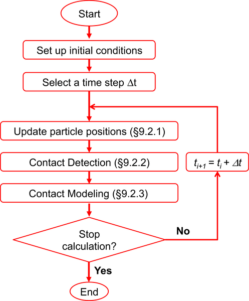
DEM generally involves cyclic calculations with a very small time increment (i.e., time step Δt). At each time step (t_i), the evolution of the system is advanced to obtain new particle positions and velocities based upon the updated forces acting on the particles. A typical DEM algorithm is illustrated in Fig. 9.1. Each calculation cycle consists of three key steps:

1. Updating particle positions (see Section 9.2.1);

2. Contact detection (Section 9.2.2);

3. Contact modeling, i.e., updating the contact forces (Section 9.2.3).

These steps are discussed in detail in the following subsections.

9.2.1. Updating Particle Positions

The motion of each particle (say particle i) is governed by Newton's second law of motion. Based upon the resultant force F_i acting on the particle i with mass m_i and moment of inertia I_i, its translational and rotational motions are determined as follows:

$m_{i} \frac{ⅆ v_{i}}{ⅆ t} = F_{i}$ $m_{i} \frac{ⅆ v_{i}}{ⅆ t} = F_{i}$

(9.1)

$I_{i} \frac{ⅆ ω_{i}}{ⅆ t} = T_{i}$ $I_{i} \frac{ⅆ ω_{i}}{ⅆ t} = T_{i}$

(9.2)

in which, v_i and ω_i are the translational and angular velocities, respectively, and T_i is the total torque. The resultant force F_i is the net force resulting from the sum of the various individual forces acting on the particles, including gravitational forces, mechanical contact forces, electrostatic forces, fluid–particle interaction forces and cohesive forces.

Numerical integration of Eqs (9.1) and (9.2) is usually achieved using a central finite difference scheme, in which a fixed time step Δt is used and new velocities and positions of each particle are calculated as follows:

$v_{i}^{t + Δ t / 2} = v_{i}^{t - Δ t / 2} + \frac{ⅆ v_{i}}{ⅆ t} Δ t$ $v_{i}^{t + Δ t / 2} = v_{i}^{t - Δ t / 2} + \frac{ⅆ v_{i}}{ⅆ t} Δ t$

(9.3a)

$ω_{i}^{t + Δ t / 2} = ω_{i}^{t - Δ t / 2} + \frac{ⅆ ω_{i}}{ⅆ t} Δ t$ $ω_{i}^{t + Δ t / 2} = ω_{i}^{t - Δ t / 2} + \frac{ⅆ ω_{i}}{ⅆ t} Δ t$

(9.3b)

and

$x_{i}^{t + Δ t} = x_{i}^{t} + v_{i}^{t + Δ t / 2} Δ t$ $x_{i}^{t + Δ t} = x_{i}^{t} + v_{i}^{t + Δ t / 2} Δ t$

(9.4a)

$θ_{i}^{t + Δ t} = θ_{i}^{t} + θ_{i}^{t + Δ t / 2} Δ t$ $θ_{i}^{t + Δ t} = θ_{i}^{t} + θ_{i}^{t + Δ t / 2} Δ t$

(9.4b)

where x_i and θ_i are the coordinates and rotational displacements of particle i, respectively.

9.2.2. Contact Detection

Once the particle positions are updated, it is necessary to detect whether new contacts between particles have been established and if any existing contact has been lost. Since DEM simulations routinely involve thousands or even millions of particles and the contact detection needs to be performed for each particle in the system in each calculation cycle, an efficient contact-searching algorithm is critical to reducing the computing time for contact detection and to improving the overall computing efficiency. For this purpose, two-phase contact searching schemes are commonly employed, which include a presorting phase and a subsequent precise contact detection phase.

The purpose of the presorting phase is to establish the neighborhood for each particle because contacts are only possible between a particle and those in the local vicinity (i.e., in its neighborhood). In other words, presorting aims to identify any potential contacting particle. The size of the neighborhood depends on the nature of the contact: for mechanical interaction that occurs when particles physically touch each other, the neighborhood can be confined to the immediate vicinity, while for interaction induced by long-range forces, such as electrostatic interaction, the neighborhood has to be large enough to ensure that all potential interactions are accounted for (Pei et al., 2015a). The presorting can be performed using two approaches: (1) a cell-based method (Fig. 9.2(a)), also known as the grid method or the boxing method, and (2) a Verlet list method (Fig. 9.2(b)).

In the cell-based method, the computation domain is divided into a number of regular cells or boxes. All particles are mapped into the cells according to their positions, and each cell has a link list of associated particles. A particle is mapped into a cell if there is any overlap between them. For example, in Fig. 9.2(a), particle 1 is only mapped into cell C1; particle 2 is mapped into two cells: B3 and C3, while particle 3 is mapped into four cells: D3, D4, E3, and E4. With the cell-based method, precise contact detection only needs to be carried out between the particle and those sharing the same cell(s) with it, i.e., those mapped into the same cell(s). For the example illustrated in Fig. 9.2(a), precise contact detection will be performed to check whether particle 1 is making contact with the particles mapped into cell C1 (i.e., 4 particles will be checked); particle 2 with those particles mapped into cells B3 and C3, and so on. It is clear that, if the cell is too large, many potential neighboring particles will be identified, which could lead to a long computing time. If the cell is too small, many particles will be mapped into multiple cells so that the particles in all these cells must be scanned, and consequently the computing time could also be very long. Hence there is an optimal cell size to achieve efficient contact detection, which can be estimated using a heuristic method or through sensitivity studies. As an approximate indication, a cell size of 3–5 particle diameters can be used to achieve a good contact searching efficiency.

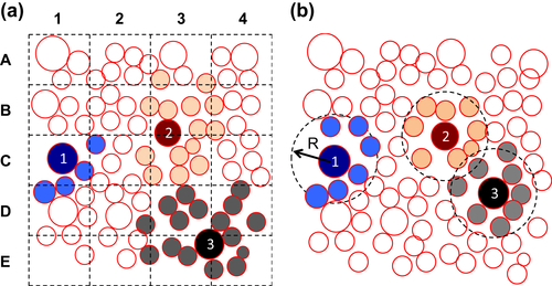
Figure 9.2 Illustration of (a) the cell-based method and (b) the Verlet list method for presorting.

In the Verlet list method, named after its originator, French physicist Loup Verlet, each particle has a list that identifies all its neighboring particles. Although no box or cell is introduced, a cut-off radius R is used to construct and maintain the list. Each particle has an associated catchment space (area in 2D; volume in 3D) of radius R, and particles are said to be its neighbors and should be added into its Verlet list if the centers of these particles are located inside the catchment space, as illustrated in Fig. 9.2(b). In contrast to the cell-based method, precise contact detection is only needed between the particles and those in its Verlet list. The cut-off distance (radius of the catchment space) needs to be carefully chosen: it should not be too large otherwise more particles are included and more time is needed for precise contact searching; it should not be so small as to exclude any potential neighboring particles.

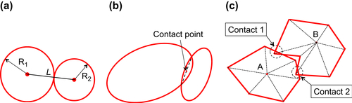
The purpose of the fine detection phase is to identify all contacts of a particle with its neighboring particles. For spherical particles, there is a mechanical contact if the distance between the centers of two particles with radius R₁ and R₂ is equal to or less than the sum of the two radii (see Fig. 9.3(a)), i.e.,

$L \leq R_{1} + R_{2}$ $L \leq R_{1} + R_{2}$

(9.5)

Contact detection for nonspherical particles (e.g., ellipsoids and polygons) is more complicated due to the more complex contact geometry. For elliptical particles in 2D, Ting et al. (1993) proposed a contact detection method in which the contact point between two elliptical particles is regarded as the midpoint of the line connecting the intersection points of the two ellipses (Fig. 9.3(b)); the intersection points can be mathematically determined using the equations defining the shapes. Similar approaches can be used for contact detection between other shapes that can be defined mathematically (Lin and Ng, 1995; Ouadfel and Rothenburg, 1999). For polygonal particles, contact detection becomes more complicated, because many types of contact may exist, including face–face, face–corner, corner–corner, and multiple contacts (see Fig. 9.3(c)). Wu and Cocks (2006) treated polygonal particles as a collection of triangles and a contact search scheme based upon each vertex was proposed. This method is able to detect each contacting vertex and multiple contacts between two particles, but it is very computationally intensive. Boon et al. (2013) proposed a contact search method for arbitrary 3D convex-shaped particles, in which the particles were constructed using an assembly of planes defined by mathematical functions, and the contact detection was performed by solving constrained minimization problems. They also showed that the computational time for contact detection for nonspherical particles is several orders of magnitude greater than that for spherical particles.

Figure 9.3 Contact detection between (a) spherical particles, (b) elliptical particles, and (c) polygonal particles.

9.2.3. Contact Modeling

Contact modeling needs to be performed once a contact between two particles is identified, so that the contact forces acting on each particle in each time increment can be updated. The mechanical interaction between two particles can be modeled using either the contact laws based upon theoretical contact mechanics (such as the Hertz theory, and the JKR model described in Chapter 8), or simplified phenomenological models, such as linear spring or spring-dashpot models. Strictly speaking, the models based upon theoretical contact mechanics can only be used to model contacts between spherical particles. For particles of irregular shape, the interaction is very complicated and no general analytical model is available. Consequently, irregular particles are often simply modeled as spheres with full contact interactions or phenomenological models are used in estimating the contact forces between those particles.

The contact laws based upon theoretical contact mechanics described in Chapter 8 can be used to model the mechanical interaction between spherical particles in DEM. For elastic spherical particles, Thornton and his coworkers (Thornton and Ning, 1997; Thornton and Yin, 1991) implemented the Hertz theory (Section 8.1.1) to model the normal force–displacement relationship and the theory of Mindlin and Deresiewicz (Section 8.1.3) for the tangential force–displacement relationship. This is often called the Hertz–Mindlin–Deresiewicz model (or the HMD model, Thornton et al., 2011), and is briefly described in Box 9.1.

For the interaction between spheres with adhesion, the JKR model (Johnson et al., 1971) discussed in Section 8.3.2.1 and the theory of Thornton (1991) can be used to describe the normal and tangential force–displacement relationships in DEM, as introduced in Box 9.2.

Box 9.1 The Hertz–Mindlin–Deresiewicz Model

Using Eq. (8.12), the normal force–displacement (F_n−δ_n) relationship between two spheres is given as

$F_{n} = \frac{4}{3} E^{*} {(R^{*})}^{1 / 2} δ_{n}^{3 / 2}$ $F_{n} = \frac{4}{3} E^{*} {(R^{*})}^{1 / 2} δ_{n}^{3 / 2}$

(9.6)

where E^∗ and R^∗ are defined in Eqs (8.6) and (8.8), respectively.

The normal stiffness k_n can be determined by differentiating Eq. (9.6) with respect to δ_n and is given as

$k_{n} = \frac{ⅆ F_{n}}{ⅆ δ_{n}} = 2 E^{*} \sqrt{R^{*} δ_{n}}$ $k_{n} = \frac{ⅆ F_{n}}{ⅆ δ_{n}} = 2 E^{*} \sqrt{R^{*} δ_{n}}$

(9.7)

indicating that the normal stiffness k_n is not a constant but varies with δ_n.

As introduced in Section 8.1.3, the interaction between frictional elastic spheres in contact under varying oblique forces was analyzed by Mindlin and Deresiewicz (1953), and solutions were obtained in the form of instantaneous compliances. As a consequence, the solutions depend not only on the current state but also the previous loading history and cannot be integrated a priori. However, through examining several loading sequences involving variations of both normal and tangential forces, some general procedural rules were identified.

The recommended procedure uses an incremental approach to update the normal force and contact radius using Eqs (9.6) and (8.12). The tangential incremental force ΔF_t is then calculated using the tangential incremental relative surface displacement Δδ_t, and the new values of F_n and a. Thornton and his coworkers (Thornton and Yin, 1991; Thornton and Randall, 1988; Thornton et al., 2011) reanalyzed the loading scenarios considered by Mindlin and Deresiewicz (1953), and showed that the tangential incremental displacement can be expressed in a general form as

$Δ δ_{t} = \frac{1}{8 G^{*} a} (\pm μ Δ F_{n} + \frac{Δ F_{t} \cdot μ Δ F_{n}}{θ})$ $Δ δ_{t} = \frac{1}{8 G^{*} a} (\pm μ Δ F_{n} + \frac{Δ F_{t} \cdot μ Δ F_{n}}{θ})$

(9.8)

where G^∗ is given by Eq. (8.25). The tangential stiffness can be obtained by rearranging Eq. (9.8):

$k_{t} = \frac{Δ F_{t}}{Δ δ_{t}} = 8 G^{*} a θ \pm μ (1 - θ) \frac{Δ F_{n}}{Δ δ_{t}}$ $k_{t} = \frac{Δ F_{t}}{Δ δ_{t}} = 8 G^{*} a θ \pm μ (1 - θ) \frac{Δ F_{n}}{Δ δ_{t}}$

(9.9)

The negative sign in Eq. (9.9) is only necessary during unloading. If ΔF_n > 0 and

| Δ δ_{t} | < \frac{μ Δ F_{n}}{8 G^{*} a}

$| Δ δ_{t} | < \frac{μ Δ F_{n}}{8 G^{*} a}$

, θ should be set to one in Eq. (9.9); otherwise, θ is given as

$θ^{3} = 1 - \frac{(F_{t} + μ Δ F_{n})}{μ F_{n}} Δ δ_{t} > 0 (loading)$ $θ^{3} = 1 - \frac{(F_{t} + μ Δ F_{n})}{μ F_{n}} Δ δ_{t} > 0 (loading)$

(9.10a)

$θ^{3} = 1 - \frac{(F_{t}^{*} - F_{t} + 2 μ Δ F_{n})}{2 μ F_{n}} Δ δ_{t} < 0 (unloading)$ $θ^{3} = 1 - \frac{(F_{t}^{*} - F_{t} + 2 μ Δ F_{n})}{2 μ F_{n}} Δ δ_{t} < 0 (unloading)$

(9.10b)

$θ^{3} = 1 - \frac{(F_{t} - F_{t}^{* *} + 2 μ Δ F_{n})}{2 μ F_{n}} Δ δ_{t} > 0 (reloading)$ $θ^{3} = 1 - \frac{(F_{t} - F_{t}^{* *} + 2 μ Δ F_{n})}{2 μ F_{n}} Δ δ_{t} > 0 (reloading)$

(9.10c)

where

F_{t}^{*}

$F_{t}^{*}$

and

F_{t}^{* *}

$F_{t}^{* *}$

specify the forces for the transitions from loading to unloading and unloading to reloading, respectively, and need to be continuously updated to account for the effect of varying normal force:

$F_{t}^{*} = F_{t}^{*} + μ Δ F_{n}$ $F_{t}^{*} = F_{t}^{*} + μ Δ F_{n}$

(9.11a)

$F_{t}^{* *} = F_{t}^{* *} - μ Δ F_{n}$ $F_{t}^{* *} = F_{t}^{* *} - μ Δ F_{n}$

(9.11b)

Box 9.2 Contact Models for Adhesive Spheres

In the JKR model (Johnson et al., 1971), the radius of the contact area a is obtained using Eq. (8.95); the applied normal force and the relative normal displacement are functions of the contact radius according to Eqs (8.97) and (8.102), i.e.,

$F_{n} = \frac{4 E^{*} a^{3}}{3 R^{*}} - 4 {(π γ E^{*} a^{3})}^{1 / 2}$ $F_{n} = \frac{4 E^{*} a^{3}}{3 R^{*}} - 4 {(π γ E^{*} a^{3})}^{1 / 2}$

(9.12)

$δ_{n} = \frac{a^{2}}{R^{*}} - 2 {(\frac{π γ a}{E^{*}})}^{1 / 2}$ $δ_{n} = \frac{a^{2}}{R^{*}} - 2 {(\frac{π γ a}{E^{*}})}^{1 / 2}$

(9.13)

The normal contact stiffness k_n can be obtained by differentiating Eqs (9.12) and (9.13) with respect to a and using

k_{n} = \frac{ⅆ F_{n}}{ⅆ δ_{n}}

$k_{n} = \frac{ⅆ F_{n}}{ⅆ δ_{n}}$

. Hence

$k_{n} = 2 E^{*} a (\frac{3 \sqrt{{\hat{F}}_{n}} - 3 \sqrt{F_{c}}}{3 \sqrt{{\hat{F}}_{n}} - \sqrt{F_{c}}})$ $k_{n} = 2 E^{*} a (\frac{3 \sqrt{{\hat{F}}_{n}} - 3 \sqrt{F_{c}}}{3 \sqrt{{\hat{F}}_{n}} - \sqrt{F_{c}}})$

(9.14)

where

{\hat{F}}_{n}

${\hat{F}}_{n}$

and F_c are defined by Eqs (8.96) and (8.106), respectively.

In order to model the tangential interaction with adhesion, Thornton (1991) developed a model that integrates the theories of Savkoor and Briggs (1977) and Mindlin and Deresiewicz (1953). In this model, the contact radius reduces with increasing tangential force F_t, i.e., the contact area shrinks as the tangential force increases. This can be visualized as the two contacting particles peeling gradually away from each other with increasing tangential force. During the peeling process, the contact radius is given as

$a^{3} = \frac{3 R^{*}}{4 E^{*}} (F_{n} + 2 F_{c} \pm \sqrt{4 F_{n} F_{c} + 4 F_{c}^{2} - \frac{F_{t}^{2} E^{*}}{4 G^{*}}})$ $a^{3} = \frac{3 R^{*}}{4 E^{*}} (F_{n} + 2 F_{c} \pm \sqrt{4 F_{n} F_{c} + 4 F_{c}^{2} - \frac{F_{t}^{2} E^{*}}{4 G^{*}}})$

(9.15)

and the tangential stiffness k_t can be obtained using the no-slip solution of Mindlin (1949) and is given as

$k_{t} = 8 G^{*} a$ $k_{t} = 8 G^{*} a$

(9.16)

The peeling process continues until the following condition is satisfied

$F_{t}^{peel} = 4 \sqrt{\frac{G^{*}}{E^{*}} (F_{n} F_{c} + F_{c}^{2})}$ $F_{t}^{peel} = 4 \sqrt{\frac{G^{*}}{E^{*}} (F_{n} F_{c} + F_{c}^{2})}$

(9.17)

and then the contact radius becomes

$a^{3} = \frac{3 R^{*}}{4 E^{*}} (F_{n} + 2 F_{c})$ $a^{3} = \frac{3 R^{*}}{4 E^{*}} (F_{n} + 2 F_{c})$

(9.18)

Thornton (1991) pointed out that peeling must occur before sliding, and there should be a smooth transition to sliding. If at the end of the peeling process the tangential force

F_{t}^{peel}

$F_{t}^{peel}$

given by (9.17) is less than the sliding force, a subsequent slip annulus is assumed to spread radially inwards and the micro-slip solution of Mindlin and Deresiewicz (1953) should then be applied until sliding occurs. The equations for this case are Eqs (9.9) to (9.12) with substitution of F_n + 2F_c for F_n. If the tangential force at the end of the peeling process is greater than the sliding force, the tangential force is immediately set to the sliding force.

Two sliding criteria are proposed to define the tangential force for sliding,

F_{t}^{slide}

$F_{t}^{slide}$

$F_{t}^{slide} = μ {\hat{F}}_{n} (1 - \frac{{\hat{F}}_{n} - F_{n}}{3 {\hat{F}}_{n}}) F_{n} < - 0.3 F_{c}$ $F_{t}^{slide} = μ {\hat{F}}_{n} (1 - \frac{{\hat{F}}_{n} - F_{n}}{3 {\hat{F}}_{n}}) F_{n} < - 0.3 F_{c}$

(9.19a)

$F_{t}^{slide} = μ (F_{n} + 2 F_{c}) F_{n} \geq - 0.3 F_{c}$ $F_{t}^{slide} = μ (F_{n} + 2 F_{c}) F_{n} \geq - 0.3 F_{c}$

(9.19b)

Figure 9.4 The typical spring-dashpot model for describing the contact interactions between particles: (a) normal contact and (b) tangential interaction.

9.2.3.1. Phenomenological Contact Models

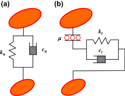
In order to determine the contact forces in DEM calculations, various phenomenological models are proposed, in which contact stiffness and energy dissipation mechanisms are incorporated to describe the interaction between particles. The phenomenological contact models are usually composed of (1) a spring to approximate elastic deformation and/or (2) a dashpot to account for the energy dissipation due to viscoelastic deformation. The spring and dashpot can be considered simultaneously in both normal and tangential directions (see Fig. 9.4). This is the so-called spring and dashpot model, also known as the Kelvin–Voigt model (Hunt and Crossley, 1975) and is widely used in non-DEM contact problems in mechanical engineering.

For systems consisting only of elastic particles, energy is primarily dissipated by friction and the particle deformation can be described using the linear stress-strain relationship shown in Figure 8.2(a). The dashpots in the normal and tangential directions shown in Fig. 9.4 can be omitted as there is no energy dissipation due to viscoelastic deformation. The contact can then be modeled using the so-called linear spring model (Thornton et al., 2011) with the normal and tangential forces being calculated by

$F_{n} = k_{n} δ_{n}$ $F_{n} = k_{n} δ_{n}$

(9.20)

$F_{t}^{new} = {\begin{matrix} F_{t}^{old} + k_{t} Δ δ_{t} & (F_{t}^{new} < μ F_{n}) \\ μ F_{n} & (F_{t}^{new} \geq μ F_{n}) \end{matrix}$ $F_{t}^{new} = {\begin{matrix} F_{t}^{old} + k_{t} Δ δ_{t} & (F_{t}^{new} < μ F_{n}) \\ μ F_{n} & (F_{t}^{new} \geq μ F_{n}) \end{matrix}$

(9.21)

The normal and tangential spring stiffnesses k_n and k_t need to be selected carefully in order to appropriately represent the interaction between two elastic bodies. Thornton et al. (2011) suggested that the normal spring stiffness k_n can be determined using the following equation:

$k_{n} = 1.2024 {(m^{1 / 2} E^{* 2} R v_{n i})}^{2 / 5}$ $k_{n} = 1.2024 {(m^{1 / 2} E^{* 2} R v_{n i})}^{2 / 5}$

(9.22)

which gives the same contact duration as the Hertz-Mindlin-Deresiewicz model for the impact of two elastic spheres. According to the Mindlin theory (Mindlin, 1949), the tangential spring stiffness k_t should have a value between

2 k_{n} / 3

$2 k_{n} / 3$

and k_n (Cundall and Strack, 1979) and can be given as a function of the Poisson's ratio υ as follows:

$k_{t} = \frac{2 (1 - υ)}{2 - υ} k_{n}$ $k_{t} = \frac{2 (1 - υ)}{2 - υ} k_{n}$

(9.23)

The normal and tangential spring stiffnesses k_n and k_t can also be calculated using Eqs (9.7) and (9.16), i.e., the Hertz theory and the “no-slip” theory of Mindlin (1949), respectively. This is referred to as the Hertz-Mindlin model (or the HM model, Thornton et al., 2011). Since k_n and k_t given by Eqs (9.7) and (9.16) are functions of the contact area (and the displacement), the HM model is essentially a nonlinear spring model.

The dashpots in Fig. 9.4 are introduced as contact damping to model the energy dissipation due to viscous deformation, in addition to friction. This is commonly known as the spring-dashpot model, in which the normal and tangential forces are calculated by

$F_{n} = k_{n} δ_{n} + c_{n} v_{n}$ $F_{n} = k_{n} δ_{n} + c_{n} v_{n}$

(9.24)

$F_{t}^{new} = {\begin{matrix} F_{t}^{old} + k_{t} Δ δ_{t} + c_{t} v_{t} & (F_{t}^{new} < μ F_{n}) \\ μ F_{n} & (F_{t}^{new} \geq μ F_{n}) \end{matrix}$ $F_{t}^{new} = {\begin{matrix} F_{t}^{old} + k_{t} Δ δ_{t} + c_{t} v_{t} & (F_{t}^{new} < μ F_{n}) \\ μ F_{n} & (F_{t}^{new} \geq μ F_{n}) \end{matrix}$

(9.25)

where c_n and c_t are the normal and tangential damping coefficients which are generally functions of the corresponding contact stiffness, i.e.,

$c_{n} = 2 β \sqrt{m^{*} k_{n}}$ $c_{n} = 2 β \sqrt{m^{*} k_{n}}$

(9.26)

$c_{t} = 2 β \sqrt{m^{*} k_{t}}$ $c_{t} = 2 β \sqrt{m^{*} k_{t}}$

(9.27)

β is the damping ratio and can be related to the normal coefficient of restitution e_n (Tsuji et al., 1992; Ting et al., 1993; Thornton et al., 2011):

$β = - \frac{\ln e_{n}}{\sqrt{π^{2} + \ln^{2} e_{n}}}$ $β = - \frac{\ln e_{n}}{\sqrt{π^{2} + \ln^{2} e_{n}}}$

(9.28)

In Eqs (9.24)–(9.27), the normal and tangential spring stiffnesses k_n and k_t can be given either by Eqs (9.7) and (9.16) or Eqs (9.22) and (9.23).

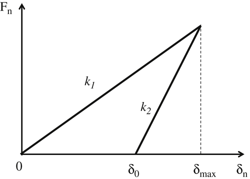
Bilinear models (see also Box 8.2) are also proposed in order to account for the effect of plastic deformation on energy dissipation. As discussed in Chapter 8, for elastoplastic materials, plastic deformation dominates the energy dissipation. It is hence reasonable that, in these hysteretic models, contact damping could be omitted. Instead, contact stiffnesses with different values are introduced for loading and unloading. This is known as the “partially latching spring” model (Walton and Braun, 1986; Walton, 1993; Thornton et al., 2013), in which the normal contact force during loading is given as

$F_{n} = k_{l} δ_{n}$ $F_{n} = k_{l} δ_{n}$

(9.29)

and during unloading,

$F_{n} = k_{2} (δ_{n} - δ_{0})$ $F_{n} = k_{2} (δ_{n} - δ_{0})$

(9.30)

where δ₀ is the relative approach when the normal force returns to zero (see Fig. 9.5),

$\frac{k_{1}}{k_{2}} = e_{n}^{2}$ $\frac{k_{1}}{k_{2}} = e_{n}^{2}$

(9.31)

$δ_{0} = δ_{\max} (1 - e_{n}^{2})$ $δ_{0} = δ_{\max} (1 - e_{n}^{2})$

(9.32)

where δ_max is the maximum relative approach.

The tangential force is calculated using Eq. (9.21) with the tangential contact stiffness (Thornton et al., 2013)

$k_{t} = k_{1} \frac{2 (1 - υ)}{2 - υ} {(1 - \frac{F_{t} - F_{t}^{*}}{μ F_{n} - - F_{t}^{*}})}^{1 / 3} for Δ F_{t} > 0$ $k_{t} = k_{1} \frac{2 (1 - υ)}{2 - υ} {(1 - \frac{F_{t} - F_{t}^{*}}{μ F_{n} - - F_{t}^{*}})}^{1 / 3} for Δ F_{t} > 0$

(9.33)

$k_{t} = k_{1} \frac{2 (1 - υ)}{2 - υ} {(1 - \frac{F_{t}^{*} - F_{t}}{μ F_{n} - F_{t}^{*}})}^{1 / 3} for Δ F_{t} < 0$ $k_{t} = k_{1} \frac{2 (1 - υ)}{2 - υ} {(1 - \frac{F_{t}^{*} - F_{t}}{μ F_{n} - F_{t}^{*}})}^{1 / 3} for Δ F_{t} < 0$

(9.34)

where ΔF_t is the tangential force increment in a given time step, and

F_{t}^{*}

$F_{t}^{*}$

is the tangential force at the instant when the relative tangential displacement reverses direction.

9.2.4. Determination of the Time Step

For cyclic calculations in DEM, it is important to select an appropriate time step. On the one hand, the time step should be as large as possible so as to increase the computing efficiency. On the other hand, it needs to be small enough that the calculations are stable and accurate, and a constant acceleration can be assumed at each time step for updating the kinematics of the particles (Section 9.2.1). A small time step will ensure that no new contacts occur in the current calculation cycle (i.e., current time step), so that the operational contacts are only those identified at the beginning of the current time step. The out-of-balance force at the end of the calculation cycle is then the resultant of the contact forces arising only from those identified contacts. The longest time for which this is true is the critical time step.

Figure 9.5 Schematic illustration of the bilinear contact model.

When a linear contact model is used (say, e.g., Eqs (9.20) and (9.21)), the critical time step can be calculated from the mass of the smallest particles in the model m_s, and the same stiffness as the normal contact stiffness k_n (Cundall, 1988; Ting et al., 1995):

$Δ t_{c} = 2 π \sqrt{\frac{m_{s}}{k_{n}}}$ $Δ t_{c} = 2 π \sqrt{\frac{m_{s}}{k_{n}}}$

(9.35)

When linear spring-dashpot models are used to describe viscous behavior, the damping ratio needs to be considered, so that the critical time step is then given as (Dziugys and Peters, 2001)

$Δ t_{c} = \frac{π}{\sqrt{\frac{k_{n}}{m_{s}} (1 - \frac{\ln^{2} e_{n}}{π^{2} + \ln^{2} e_{n}})}}$ $Δ t_{c} = \frac{π}{\sqrt{\frac{k_{n}}{m_{s}} (1 - \frac{\ln^{2} e_{n}}{π^{2} + \ln^{2} e_{n}})}}$

(9.36)

For DEM modeling with nonlinear models, a widely used approach to determination of the critical time step is based on the frequency of the Rayleigh wave, a kind of surface acoustic wave which travels on solids. In particular, the time step used must be smaller than the time for the Rayleigh wave to propagate through the smallest particle in the assembly. This leads to a critical time step given by

$Δ t_{c} = \frac{π d_{min}}{2 λ} \sqrt{\frac{ρ_{s}}{G}}$ $Δ t_{c} = \frac{π d_{min}}{2 λ} \sqrt{\frac{ρ_{s}}{G}}$

(9.37)

where

$λ = 0.1631 υ + 0.8766$ $λ = 0.1631 υ + 0.8766$

(9.38)

d_min, ρ_s, G, and υ are respectively the diameter, true density, shear modulus, and Poisson's ratio of the smallest particle in the particle assembly.

9.2.5. Determination of DEM Parameters

It can be seen from the discussion in Section 9.2.3 that several key parameters need to be defined for contact modeling in DEM, including the normal and tangential contact stiffnesses k_n and k_t and friction coefficient μ. The contact stiffnesses can be related to the material intrinsic properties, such as Young's Modulus E, Poisson's ratio υ, true density ρ, and particle size d, which can be obtained either from materials handbooks or through experimental characterization using advanced techniques such as nano-indentation and atomic force microscopy (AFM). Direct measurement of the friction coefficient μ between particles and with other surfaces is very difficult, even with advanced techniques such as AFM and use of a nano-tribometer. Alternative approaches to determining the friction coefficient include inferring it from single-particle impact experiments using the theories discussed in Chapter 8 (Lorenz et al., 1997; Foerster et al., 1994; Gorham and Kharaz, 2000) or from the friction measurement of bulk solids (Li et al., 2005). Table 9.1 lists some friction coefficients reported in the literature.

Table 9.1

Friction Coefficients for Various Materials Reported in the Literature

Materials	μ	References
Acrylic ball–acrylic ball	0.096 ± 0.006	Lorenz et al. (1997)
Acrylic ball–aluminum plate	0.140	Mullier et al. (1991)
Aluminum oxide sphere–aluminum alloy lead plate	0.180	Gorham and Kharaz (2000)
Aluminum oxide sphere–glass plate	0.092	Gorham and Kharaz (2000)
Cellulose acetate–cellulose acetate ball	0.250 ± 0.020	Foerster et al. (1994)
Cellulose acetate ball–cellulose acetate ball	0.220∼0.330	Mullier et al. (1991)
Fresh glass ball–aluminum plate	0.131 ± 0.007	Lorenz et al. (1997)
Fresh glass ball–fresh glass ball	0.048 ± 0.006	Lorenz et al. (1997)
Glass ball–glass plate	0.155	Li et al. (2005)
Glass ball–perspex plate	0.133	Li et al. (2005)
Nylon ball–nylon ball	0.175 ± 0.100	Labous et al. (1997)
Polystyrene ball–polystyrene ball	0.189 ± 0.009	Lorenz et al. (1997)
Radish seeds–aluminum plate	0.190	Mullier et al. (1991)
Soda lime glass ball–soda lime glass ball	0.092 ± 0.006	Foerster et al. (1994)
Spent glass ball–spent glass ball	0.177 ± 0.020	Lorenz et al. (1997)
Spent glass ball–spent glass ball (stationary)	0.126 ± 0.014	Lorenz et al. (1997)
Spent glass ball–aluminum plate	0.126 ± 0.009	Lorenz et al. (1997)
Stainless steel ball–stainless steel ball	0.099 ± 0.008	Lorenz et al. (1997)
Steel ball–steel plate	0.214	Li et al. (2005)

9.3. Data Analysis

From cyclic calculations, detailed microscopic information on each particle at each time step can be obtained, including positions, velocities, accelerations, and contact forces. Normally this is just the beginning of the analysis process, and much more insight into particulate processes can be gained by appropriate choices of further data analysis techniques. The ultimate goal is to relate the macroscopic performance to the intrinsic particle properties and to the microscopic behavior at the particle level. In this section, some characteristics of particle systems that can be obtained from DEM data are introduced.

9.3.1. Macroscopic Deformation Patterns

Knowing the position of each particle at each time step, the evolution of macroscopic deformation patterns can be readily obtained by displaying each particle. To enhance the visualization of the deformation pattern, particles can be color coded either according to their initial position or their distinctive features (such as density or size). The former is generally employed to explore the deformation patterns of particles during shearing or flow, while the latter offers good visual demonstrations of particle mixing or segregation. Figs 9.6 and 9.7 present some typical examples in which color-coded particle bands are employed to show the deformation patterns. Some examples in which colors are used to indicate particles of different properties are presented in Fig. 9.8. In addition to static representations of this kind, successive “frames” can be built up into animations, so demonstrating the system dynamics.

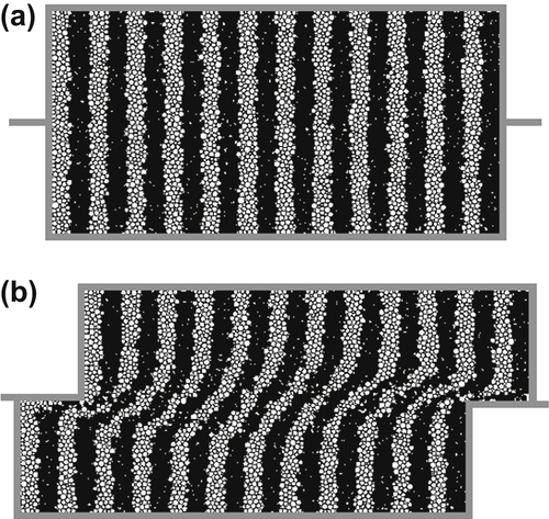
Figure 9.6 Deformation pattern of DEM specimen in a direct shear test observed using color-coded particle bands (Zhang, 2003). The deformation of the particle system under shear is clearly shown; (a) before shearing, and (b) end of shearing.

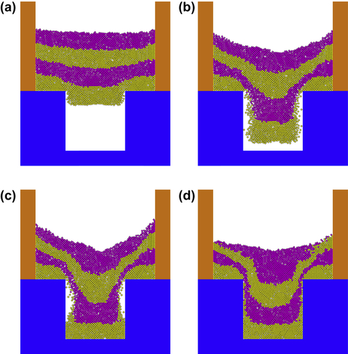
Figure 9.7 Powder flow patterns during die filling obtained from DEM analysis (Guo et al., 2009b), in which bands of particles are color-coded according to their initial positions. (a) t = 8.5 ms, (b) t = 17.0 ms, (c) t = 20.5 ms, and (d) t = 56.2 ms.

9.3.2. Force Transmission Network

Contact forces between particles at each time step can be displayed to show the force transmission patterns (or contact force network) at various time instants. An example is presented in Fig. 9.9, in which the contact force is visualized as a solid line connecting the centers of the two contacting spheres (indicating the direction of the contact force), with the thickness of the line representing either the magnitude of the contact force or the ratio of the contact force to the average contact force in the system. This allows the contact force network to be classified into the strong force network formed by contact forces more than the average contact force, and the weak force network showing the contact forces less than the average. Different shades of gray or different colors can then be used to visualize these two sub-networks, as shown in Fig. 9.9, in which the strong force network is shown in bold and the weak force network is shown in gray. Using this approach, the macroscopic force transmission in the system can be clearly visualized and related to forces at the single particle level.

Figure 9.8 Packing patterns of DEM specimen during die filling observed using color-coded particles; the “shoe” containing the particles moves from right to left. Yellow (light gray in print versions) represents small particles and magenta (dark gray in print versions) represents the large particles. Segregation during die filling is clearly shown (Guo et al., 2010); (a) before die filling and (b) after die filling.

9.3.3. Packing Density Distribution

In a number of applications, such as packing of particles in a container, it is of practical importance to know the density distribution. This can be readily achieved from the DEM analysis, as the positions of individual particles are explicitly determined at each time step. Two approaches can be used to obtain the density distribution: (1) the box method and (2) the Voronoi cell method (after Georgy Voronoy, Ukrainian/Russian mathematician).

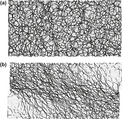
Figure 9.9 Force transmission patterns during the direct shear test obtained from DEM analysis (Zhang, 2003); (a) before shearing, and (b) during shearing.

In the box method, the space occupied by the particle system is divided into a number of grids. The packing density in each box can be determined by treating each box as a subset of the whole particle system and using the void fraction or solid fraction defined by Eqs (2.17) and (2.18), respectively, as illustrated in Fig. 9.10. The solid fraction in the highlighted box is defined as either the ratio of the volume of the shaded particles to the volume of the box in 3D, or the ratio of the area of particles to that of the box in 2D. Knowing the packing density in each box, the spatial distribution of the packing density can then be obtained, which is generally presented in contour plots as illustrated in Fig. 9.11. It is to be expected that the calculated density (and solid fraction and void fraction) will depend to some extent on the box size, as shown in Fig. 9.10. Generally, the box size must be larger than the size of the largest particle in the system, and sensitivity studies need to be performed to select an appropriate box size.

In the Voronoi cell method, the particle system is divided into a number of cells, each of which is a polyhedron containing only one particle, such that the surface of the cell is equidistant from the surface of the particle and the surfaces of its nearest neighbors. The number of close neighbors therefore determines the number of faces, as shown in Fig. 9.12. For each Voronoi cell, the volume can be calculated and the relative density can be determined as the ratio of the sphere volume to that of the cell, from which the density distribution can then be obtained. An example of the density distribution obtained using the Voronoi cell method is given in Fig. 9.13. The packing density using this method requires no choice about scale of scrutiny; hence, the Voronoi cell approach is in principle a superior method for determination of packing density distributions from DEM calculations.

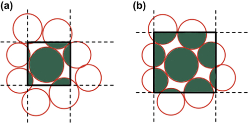
Figure 9.10 The box method for calculating density distributions; (a) with small box size; (b) with large box size.

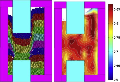
Figure 9.11 Particle packing pattern for a powder transfer operation and the resulting solid fraction distribution determined using the box method, from 2D DEM analysis (Coube et al., 2005).

Despite the inherent superiority of the Voronoi cell method, the box method is easier to implement and has the additional advantage that it enables distributions of other particle system characteristics to be obtained simultaneously using the same box configurations. For example, it is possible to obtain the distributions of the average particle rotation, ϖ, of the sample using the same box method as used for determining the packing density distribution. Here ϖ is defined as the average rotation of all the particles in each box:

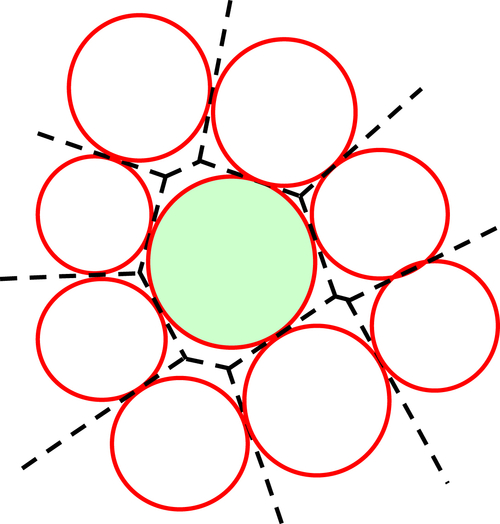
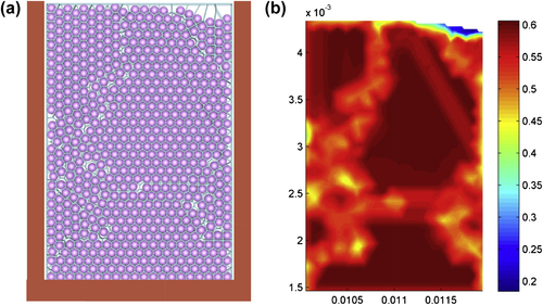
Figure 9.13 Packing of particles in a container: (a) the particle packing pattern and associated Voronoi cells and (b) the solid fraction distributions determined using the Voronoi cell method.

$〈 θ 〉 = \frac{\sum_{i = 1}^{C} ω_{i}}{n_{p}}$ $〈 θ 〉 = \frac{\sum_{i = 1}^{C} ω_{i}}{n_{p}}$

(9.39)

where ω_i is the rotation of particle i and n_p is the total number of particles in each box.

9.3.4. Radial Distribution Function

Particle packing structures can also be described statistically using the radial distribution function (RDF), g(r), i.e., the probability of finding a particle at a distance r away from a reference particle. The RDF can be evaluated by counting how many particles have their centres within a distance of r to r + Δr away from the reference particle (see Fig. 9.14), i.e., the number of particles with their centres in a spherical shell of radius r and thickness Δr. The RDF for a 2D inhomogeneous system is defined as:

$g (r) = \frac{n (r)}{2 π r \bar{n} Δ r}$ $g (r) = \frac{n (r)}{2 π r \bar{n} Δ r}$

(9.40)

and, for a 3D system

$g (r) = \frac{n (r)}{4 π r^{2} \bar{n} Δ r}$ $g (r) = \frac{n (r)}{4 π r^{2} \bar{n} Δ r}$

(9.41)

where

r is the distance from the reference particle;

n(r) is the mean number of particles within a ring (2D) or a spherical shell (3D) of thickness Δr at a distance of r;

\bar{n}

$\bar{n}$

is the mean number density of particles.

From DEM data, the RDF can be determined by first calculating the distances between all particle pairs and then determining the distribution of that distance. Figure 9.15 shows an example of the RDF for a simple packing of particles with the same particle size and the same electrostatic charge, indicating the variation of the number density of particles with separation distance.

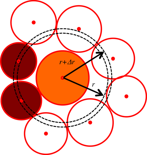
Figure 9.14 Definition of radial distribution function.

Figure 9.15 The particle packing pattern (a) and corresponding RDF (b) of charged particles obtained using DEM (Pei et al., 2015a).

9.3.5. Coordination Number

The coordination number is another important statistical parameter that can be used to characterize the packing structure of a particle system. It indicates the number of contacts of a reference particle. As illustrated in Fig. 9.16, Particle 1 has no contact, so its coordination number is 0; particles 2, 5, 6, and 7 have two contacts each, so their coordination number is 2; particles 3, 4, 8, 9, and 10 have a coordination number of 3 as they have three contacts each; particle 11 has only one contact, so its coordination number is 1.

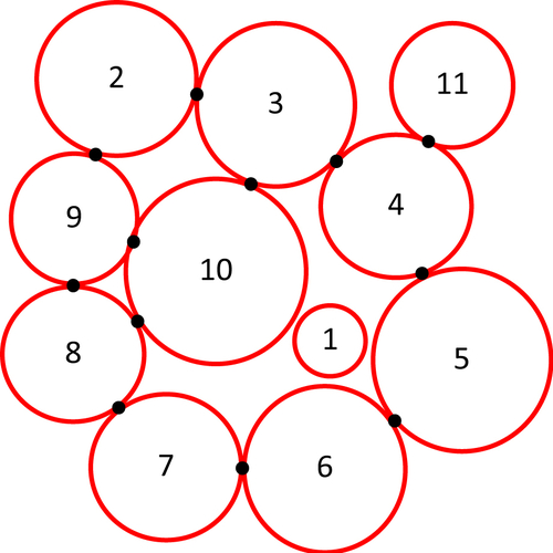
For a particle system, the average coordination number Z is defined as:

$Z = \frac{2 N_{C}}{n_{p}}$ $Z = \frac{2 N_{C}}{n_{p}}$

(9.42)

where N_C is the total number of contacts and n_p is the total number of particles. For the example illustrated in Fig. 9.16, the total number of contacts (shown as black dots), N_C, is 12 and the average coordination number is therefore 2.18.

Zhang (2003) argued that particles which have no contacts with others (such as particle 1 in Fig. 9.16), and particles which have only one contact with their neighboring particles (e.g., particle 11 in Fig. 9.16) cannot make any contribution to the mechanical properties of the particle system (i.e., the removal of particles 1 and 11 in the system illustrated in Fig. 9.16 will not significantly affect the mechanical behavior of the whole). Hence, a mechanical coordination number was introduced and defined as:

$Z_{m} = \frac{2 N_{C} - n_{1}}{(n_{p} - n_{1} - n_{0})}, Z_{m} \geq 2$ $Z_{m} = \frac{2 N_{C} - n_{1}}{(n_{p} - n_{1} - n_{0})}, Z_{m} \geq 2$

(9.43)

where n₁ and n₀ are the numbers of particles with one and no contacts, respectively. For the example given in Fig. 9.16, N_C = 12, n₁ = n₀ = 1, n_p = 11, so Z_m = 2.56.

The coordination number reflects the degree of connection between particles so it can be used to evaluate the packing of the systems, in applications such as force transmission and tensile strength (Cundall and Strack, 1979). Not surprisingly, published data show that the average coordination number has a strong correlation with measurements of particle packing density such as the solid fraction or void fraction (Oda, 1977), increasing for higher packing density (solid fraction). For example, for ordered packing of monosized particles, the correlation between the average coordination number and the solid fraction D can be approximated using one of the following empirical expressions, among many others (German and Park, 2008):

$Z = \frac{π}{1 - D}$ $Z = \frac{π}{1 - D}$

(9.44)

$Z = 14 - 10.4 {(1 - D)}^{0.38}$ $Z = 14 - 10.4 {(1 - D)}^{0.38}$

(9.45)

9.3.6. Microstructural Characteristics

The macroscopic properties of a particulate system depend on its microstructure, which can be described in different ways. Some microstructural properties are scalars, i.e. they have magnitude but no direction. An example is solid fraction. Many characteristics of a particle system, however, are vectors, i.e., they have both magnitude and direction, examples including contact force, displacement and velocity of particles. Two particle systems of the same material and the same solid fraction may show very different mechanical responses if they have different microstructures (Oda, 1977; Oda et al., 1980). A further complication is isotropy. A particle system is isotropic with respect to a certain property if the values of that property are identical in all directions. When a property has different values in different directions, the system is said to be anisotropic with respect to that property. Using DEM data, two parameters can be determined which characterize the microstructure of a particle system: (1) the fabric tensor and (2) the contact normal orientations. Both are based upon the distribution of contact normal vectors that determine the structural anisotropy of a particle system. If the distribution of the contact normal vectors is random and can be approximated using a uniform distribution, the particle system in effect possesses an isotropic structure. If the distribution is non-uniform, the structure is then anisotropic.

For assemblies of discs or spheres, the fabric tensor ϕ_ij characterizes the structural anisotropy using the contact normals n_i and n_j (Satake, 1982):

$φ_{i j} = 〈 n_{i} n_{j} 〉 = \frac{1}{2 N_{C}} \sum_{1}^{2 N_{C}} n_{i} n_{j}$ $φ_{i j} = 〈 n_{i} n_{j} 〉 = \frac{1}{2 N_{C}} \sum_{1}^{2 N_{C}} n_{i} n_{j}$

(9.46)

In order to obtain a complete characterization of the microstructure, a second order fabric tensor was proposed by Oda et al. (1980),

$F_{i j} = \frac{2 N_{C} \bar{R}}{V} φ_{i j}$ $F_{i j} = \frac{2 N_{C} \bar{R}}{V} φ_{i j}$

(9.47)

where

\bar{R}

$\bar{R}$

is the mean particle radius and V is the volume of the particle system.

Contact normal orientations can be used to describe load-induced anisotropy. From the DEM data, the distribution of the orientations of the contact normals can be obtained by plotting a histogram of the proportion of contact normals in a series of adjacent orientation classes that partition the full orientation space (i.e., a unit circle), as shown in Fig. 9.17. In order to construct such a diagram, each contact is interrogated to find out which of the partitioned bands (i.e., contact normal directions) its inclination belongs to. If it falls into band i, the total contact number for the band i is increased by one. After all contacts are examined, the total contact number of each band is divided by the total number of contacts in the whole system to obtain the radial coordinate as follows:

Figure 9.17 Typical patterns of the contact normal orientation distribution (Zhang, 2003); (a) Isotropic distribution, (b) Weak anisotropy, and (c) Strong anisotropy.

$r_{i} = \frac{n_{C i}}{N_{C}}$ $r_{i} = \frac{n_{C i}}{N_{C}}$

(9.48)

where n_Ci is the total number of contacts mapped into band i.

The same method can also be used to obtain the distribution of contact normals weighted by the magnitude of the contact normal force, in which the total normal force accumulated for each band is normalized by the total normal force of the whole system. Hence, the radial coordinate p_i for band i is given as:

$p_{i} = \frac{\sum_{1}^{n_{C i}} F_{n}^{i}}{\sum F_{n}}$ $p_{i} = \frac{\sum_{1}^{n_{C i}} F_{n}^{i}}{\sum F_{n}}$

(9.49)

where

F_{n}^{i}

$F_{n}^{i}$

is the contact normal force mapped into band i.

Some typical patterns of the contact normal orientation distribution are illustrated in Fig. 9.17. If the contact normal orientation distribution is isotropic, its shape is close to a circle (Fig. 9.17(a)). With increasing anisotropy (i.e., from weak anisotropy shown in Fig. 9.17(b) to strong anisotropy shown in Fig. 9.17(c)), the shape mutates to a peanut shape.

9.4. Applications

Since the first publication on DEM in 1979, the method has gained in popularity in a wide range of disciplines and fields, including chemical engineering, mechanical engineering, civil engineering, physics, agriculture, astrophysics and mathematics. It has become a powerful way of simulating particle systems: not only dispersed systems in which the particle–particle interactions are collisional, but also compact systems of particles with multiple enduring contacts. It can be used to obtain data that are normally inaccessible to physical experimentation and to perform rigorous and revealing parametric studies, including those of the “what if?” kind. There is a large collection of publications on the applications of DEM, including a review article of Zhu et al. (2008) and a series of special issues on DEM modeling (Thornton, 2000, 2008, 2009; Wu, 2012a, 2012b).

DEM is a powerful tool for providing dynamic information at a microscopic level, e.g., individual particle trajectories and transient interaction forces. Such information is essential to understanding of the underlying physics of particulate materials. For example, DEM has been widely employed to investigate processes including:

• Heap formation (Luding, 1997; Baxter et al., 1997; Matuttis et al., 2000; Smith et al., 2001; Zhou et al., 2003; Tüzün et al., 2004; Fazekas et al., 2005), for which DEM was used to explore how particle properties (shape, size, size distribution, friction, density, and mechanical properties) affect the angle of repose; to analyze force transmission in heap formation and to calculate the pressure distribution at the bottom of the heap; and to examine the effects of particle properties on segregation during heap formation.

• Particle packing. DEM can be used to analyze the packing of particles of different sizes and shapes, such as fine particles, cohesive particles, and wet particles (e.g., Yang et al., 2003, 2008; Li et al., 2005). It can be used to explore the microstructure (connectivity, coordination member, RDF, porosity, and density distributions) and analyze the force and stress transmission in a packed particle bed. It can also be used to explore how single particle properties (size, shape, mechanical properties) and interfacial properties (surface energy and friction) affect the microstructure and packing behavior.

• Powder compaction. DEM can be used to simulate bulk deformation of packed particle systems under consolidation and to explore the microstructural characteristics, stress transmission and density variations during powder compaction (see, e.g., Ng, 1999; Martin et al., 2006).

• Shear tests. DEM can be used to model deformation behavior of particle systems under different shearing conditions, such as direct shear, simple shear, and biaxial shear, and to explore the mechanics of granular materials under shear deformation at microscopic and macroscopic levels, such as stress transmission, shear band formation, and dilation (Thornton and Zhang, 2003, 2006; Zhang and Thornton, 2007; Rock et al., 2008).

• Hopper flow. DEM can be used to simulate the dynamics of particle flow in and from containers such as hoppers, from which the force transmission to the hopper walls, particle velocities inside the hopper, and mass flow rate of the particles discharging from the hopper can all be determined. DEM can also be used to analyze the flow pattern (mass flow, core flow) and to guide the hopper design for a given material (see, e.g., Kohring et al., 1995; Langston et al., 1997; Ketterhagen et al., 2007, 2008).

• Powder flow. Similarly to modeling hopper flow, DEM has been proved to be useful for modeling powder flow in processing devices such as the V-mixer (Kuo et al., 2002; Lemieux et al., 2008), rotating drums (Dury et al., 1998; Mishra et al., 2002), and die filling and powder transfer (Wu et al., 2003; Coube et al., 2005; Wu and Cocks, 2006; Wu, 2008; Guo et al., 2009a, 2009b; Bierwisch et al., 2009). From DEM analysis, not only the flow patterns but also quantitative information on flow rate, flow velocity, solids fluxes and stress and force distributions can be obtained. These can be used to guide process design and optimization.

• Mixing and segregation. DEM is a robust method for analyzing mixing and segregation of powder mixtures as the motion of each particle in the system is explicitly determined. DEM has been used extensively to explore mixing of particles and to analyze segregation in processes such as in a rotating drum (Dury et al., 1998), during die filling (Guo et al., 2009a, 2010), and in vibrating beds (Zeilstra et al., 2006, 2008), induced by air flow, size and density differences.

• Electrostatics in particle systems. With the implementation of a contact electrification model (Pei et al., 2013, 2014) and incorporation of electrostatic interactions (with proper consideration of contact detection for particle systems with long-range interaction (Pei et al., 2015a)), DEM can be used to analyze how particles become charged during handling and processing and how the electrostatic charge affects their subsequent behavior. It can also be used to investigate the uniformity of charge distribution on irregularly shaped particles (Pei et al., 2015b) with potential to model electrostatics in particle systems for real applications.

..................Content has been hidden....................

You can't read the all page of ebook, please click here login for view all page.

Table of Contents for Chapter 9. Discrete Element Methods

Create new playlist

Sign In

Sign Up

Abstract

Keywords

9.1. Hard-Sphere and Soft-Sphere DEMs

9.2. The Principle of DEM

9.2.1. Updating Particle Positions

9.2.2. Contact Detection

9.2.3. Contact Modeling

9.2.3.1. Phenomenological Contact Models

9.2.4. Determination of the Time Step

9.2.5. Determination of DEM Parameters

9.3. Data Analysis

9.3.1. Macroscopic Deformation Patterns

9.3.2. Force Transmission Network

9.3.3. Packing Density Distribution

9.3.4. Radial Distribution Function

9.3.5. Coordination Number

9.3.6. Microstructural Characteristics

9.4. Applications

Table of Contents for
Chapter 9. Discrete Element Methods